昇思MindSpore学习笔记7--函数式自动微分

摘要：

介绍了昇思MindSpore神经网络训练反向传播算法中函数式自动微分的使用方法和步骤。包括构造计算函数和神经网络、grad获得微分函数，以及如何处理停止渐变、获取辅助数据等内容。

一、概念要点

神经网络训练主要使用反向传播算法：

        准备模型预测值logits与正确标签label

        损失函数loss function计算loss

        反向传播计算梯度gradients

        更新模型参数parameters

自动微分

        计算可导函数在某点处的导数值

        将复杂的数学运算分解为一系列简单的基本运算

MindSpore函数式自动微分接口

        grad

        value_and_grad

二、环境准备

安装minspore模块

!pip uninstall mindspore -y
!pip install -i https://pypi.mirrors.ustc.edu.cn/simple mindspore==2.3.0rc1

导入numpy、minspore、nn、ops等相关模块

import numpy as np
import mindspore
from mindspore import nn
from mindspore import ops
from mindspore import Tensor, Parameter

三、函数与计算图

计算图是用图论语言来表示数学函数。

深度学习框架用来表达神经网络模型。

以下图为例构造计算函数和神经网络。

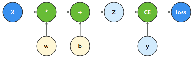
在这个模型中，x为输入，z为预测值，y为目标值，w和b是需要优化的参数。

根据计算图表达的计算过程，构造计算函数。

binary_cross_entropy_with_logits

        损失函数，计算预测值z和目标值y之间的二值交叉熵损失。

x = ops.ones(5, mindspore.float32)  # input tensor
y = ops.zeros(3, mindspore.float32)  # expected output
w = Parameter(Tensor(np.random.randn(5, 3), mindspore.float32), name='w') # weight
b = Parameter(Tensor(np.random.randn(3,), mindspore.float32), name='b') # bias

def function(x, y, w, b):
    z = ops.matmul(x, w) + b
    loss = ops.binary_cross_entropy_with_logits(z, y, ops.ones_like(z), ops.ones_like(z))
return loss

loss = function(x, y, w, b)
print(loss)

输出：

1.5375124

四、微分函数与梯度计算

优化模型参数需要对参数w、b求loss的导数：和

调用mindspore.grad函数获得function的微分函数。

 注：grad获得微分函数是一种函变换，即输入为函数，输出也为函数。

grad_fn = mindspore.grad(function, (2, 3))

mindspore.grad函数的两个入参：

fn： 求导函数。

grad_position：求导参数的索引位置。

参数 w和b在function入参对应的位置为(2, 3)。

执行微分函数获得w、b对应的梯度。

grads = grad_fn(x, y, w, b)
print(grads)

输出：

(Tensor(shape=[5, 3], dtype=Float32, value=
[[ 2.72169024e-01,  2.06588134e-01,  2.85908401e-01],
 [ 2.72169024e-01,  2.06588134e-01,  2.85908401e-01],
 [ 2.72169024e-01,  2.06588134e-01,  2.85908401e-01],
 [ 2.72169024e-01,  2.06588134e-01,  2.85908401e-01],
 [ 2.72169024e-01,  2.06588134e-01,  2.85908401e-01]]), 
Tensor(shape=[3], dtype=Float32, value=
 [ 2.72169024e-01,  2.06588134e-01,  2.85908401e-01]))

五、Stop Gradient停止渐变

消除某个Tensor对梯度的影响，或实现对某个输出项的梯度截断

通常情况下，求导函数的输出只有loss一项。

微分函数会对参数求所有输出项的导数。

function_with_logits修改原function支持同时输出loss和z

获得自动微分函数并执行。

def function_with_logits(x, y, w, b):
    z = ops.matmul(x, w) + b
    loss = ops.binary_cross_entropy_with_logits(z, y, ops.ones_like(z), ops.ones_like(z))
    return loss, z
grad_fn = mindspore.grad(function_with_logits, (2, 3))
grads = grad_fn(x, y, w, b)
print(grads)

输出：

(Tensor(shape=[5, 3], dtype=Float32, value=
[[ 1.27216899e+00,  1.20658815e+00,  1.28590846e+00],
 [ 1.27216899e+00,  1.20658815e+00,  1.28590846e+00],
 [ 1.27216899e+00,  1.20658815e+00,  1.28590846e+00],
 [ 1.27216899e+00,  1.20658815e+00,  1.28590846e+00],
 [ 1.27216899e+00,  1.20658815e+00,  1.28590846e+00]]),
 Tensor(shape=[3], dtype=Float32, value=
 [ 1.27216899e+00,  1.20658815e+00,  1.28590846e+00]))

w、b对应的梯度值变了。

使用ops.stop_gradient接口屏蔽z对梯度的影响

def function_stop_gradient(x, y, w, b):
    z = ops.matmul(x, w) + b
    loss = ops.binary_cross_entropy_with_logits(z, y, ops.ones_like(z), ops.ones_like(z))
    return loss, ops.stop_gradient(z)
grad_fn = mindspore.grad(function_stop_gradient, (2, 3))
grads = grad_fn(x, y, w, b)
print(grads)

输出：

(Tensor(shape=[5, 3], dtype=Float32, value=
[[ 2.72169024e-01,  2.06588134e-01,  2.85908401e-01],
 [ 2.72169024e-01,  2.06588134e-01,  2.85908401e-01],
 [ 2.72169024e-01,  2.06588134e-01,  2.85908401e-01],
 [ 2.72169024e-01,  2.06588134e-01,  2.85908401e-01],
 [ 2.72169024e-01,  2.06588134e-01,  2.85908401e-01]]),
 Tensor(shape=[3], dtype=Float32, value=
 [ 2.72169024e-01,  2.06588134e-01,  2.85908401e-01]))

此时w、b对应的梯度值与初始function求得的梯度值一致。

六、Auxiliary data辅助数据

函数除第一个输出项外的其他输出。

通常会将loss设置为函数的第一个输出，其他的输出即为辅助数据。

grad和value_and_grad的has_aux参数

设置True，自动实现stop_gradient，返回辅助数据，同时不影响梯度计算的效果。

下面仍使用function_with_logits，配置has_aux=True，并执行。

grad_fn = mindspore.grad(function_with_logits, (2, 3), has_aux=True)
grads, (z,) = grad_fn(x, y, w, b)
print(grads, z)

输出：

(Tensor(shape=[5, 3], dtype=Float32, value=
[[ 2.72169024e-01,  2.06588134e-01,  2.85908401e-01],
 [ 2.72169024e-01,  2.06588134e-01,  2.85908401e-01],
 [ 2.72169024e-01,  2.06588134e-01,  2.85908401e-01],
 [ 2.72169024e-01,  2.06588134e-01,  2.85908401e-01],
 [ 2.72169024e-01,  2.06588134e-01,  2.85908401e-01]]),
 Tensor(shape=[3], dtype=Float32, value=
 [ 2.72169024e-01,  2.06588134e-01,  2.85908401e-01]))
 [1.4928596  0.48854822 1.7965223 ]

此时w、b 对应的梯度值与初始function求得的梯度值一致，

同时z能够作为微分函数的输出返回。

七、神经网络梯度计算

下面通过继承nn.Cell构造单层线性变换神经网络

利用函数式自动微分来实现反向传播。

使用mindspore.Parameter封装w、b模型参数作为内部属性

在construct内实现相同的Tensor操作。

# Define model
class Network(nn.Cell):
    def __init__(self):
        super().__init__()
        self.w = w
        self.b = b
​
    def construct(self, x):
        z = ops.matmul(x, self.w) + self.b
        return z

# Instantiate model
model = Network()
# Instantiate loss function
loss_fn = nn.BCEWithLogitsLoss()

使用函数式自动微分需要将神经网络和损失函数的调用封装为一个前向计算函数。

# Define forward function
def forward_fn(x, y):
    z = model(x)
    loss = loss_fn(z, y)
    return loss

使用value_and_grad接口获得微分函数，用于计算梯度。

Cell封装神经网络模型，模型参数为Cell的内部属性，不需要使用grad_position指定对函数输入求导，因此将其配置为None。

使用model.trainable_params()方法从weights参数取出可以求导的参数。

grad_fn = mindspore.value_and_grad(forward_fn, None, weights=model.trainable_params())
loss, grads = grad_fn(x, y)
print(grads)

输出：

(Tensor(shape=[5, 3], dtype=Float32, value=
[[ 2.72169024e-01,  2.06588134e-01,  2.85908401e-01],
 [ 2.72169024e-01,  2.06588134e-01,  2.85908401e-01],
 [ 2.72169024e-01,  2.06588134e-01,  2.85908401e-01],
 [ 2.72169024e-01,  2.06588134e-01,  2.85908401e-01],
 [ 2.72169024e-01,  2.06588134e-01,  2.85908401e-01]]),
 Tensor(shape=[3], dtype=Float32, value=
 [ 2.72169024e-01,  2.06588134e-01,  2.85908401e-01]))

执行微分函数，可以看到梯度值和前文function求得的梯度值一致。