DAY 46 通道注意力(SE注意力)
知识点回顾:
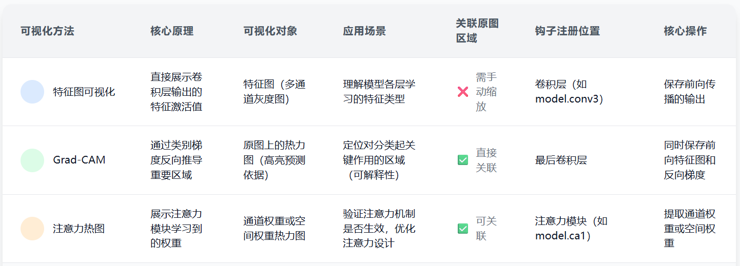
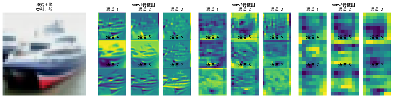
- 不同CNN层的特征图:不同通道的特征图
- 什么是注意力:注意力家族,类似于动物园,都是不同的模块,好不好试了才知道。
- 通道注意力:模型的定义和插入的位置
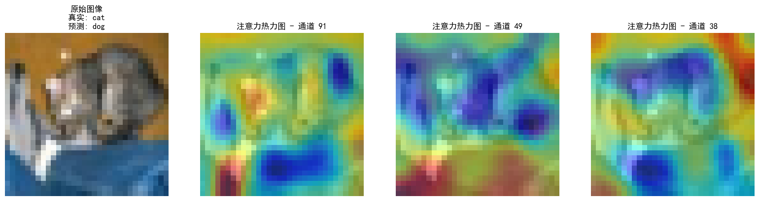
- 通道注意力后的特征图和热力图
内容参考
作业:
- 今日代码较多,理解逻辑即可
- 对比不同卷积层特征图可视化的结果(可选)
ps:
- 我这里列出来的是通道注意力中的一种,SE注意力
- 为了保证收敛方便对比性能,今日代码训练轮数较多,比较耗时
- 目前我们终于接触到了模块,模块本质上也是对特征的进一步提取,整个深度学习就是在围绕特征提取展开的,后面会是越来越复杂的特征提取和组合步骤
- 新增八股部分,在本讲义目录中可以看到----用问答的形式记录知识点
import torch
import torch.nn as nn
import torch.nn.functional as F
import torchvision.transforms as transforms
from PIL import Image
import matplotlib.pyplot as plt
import numpy as np
import requests
from io import BytesIO

# 0. 设备选择
device = torch.device("cuda" if torch.cuda.is_available() else "cpu")
print(f"Using device: {device}")

# 1. 知识点回顾与准备
# --------------------------------------------------------------------------------
# 不同CNN层的特征图:
# CNN通过一系列卷积、激活和池化操作从输入图像中提取层次化特征。
# 浅层(靠近输入的层)通常学习边缘、角点、颜色等低级特征。
# 深层(靠近输出的层)则组合低级特征形成更复杂、更抽象的高级特征,如物体部件或整个物体。
# 每个卷积层的输出包含多个通道(channel),每个通道可以看作是一个特征图(feature map),
# 代表了输入图像在某种特定模式上的响应。

# 什么是注意力:
# 注意力机制模仿人类视觉系统,使模型能够动态地关注输入数据中更相关的部分,而忽略不重要的部分。
# 它不是一个单一的算法,而是一个“家族”或“模块化思想”,有多种实现方式(如空间注意力、通道注意力、自注意力等)。
# 选择哪种注意力模块,以及如何将其集成到现有模型中,往往需要实验来验证其效果。

# 通道注意力:
# 通道注意力机制旨在学习不同特征通道之间的重要性。
# 它会为每个通道生成一个权重,然后用这些权重去重新调整(recalibrate/rescale)原始的特征图。
# 重要的通道会被赋予更高的权重,不那么重要的通道则会被抑制。
# SEBlock (Squeeze-and-Excitation Block) 是一个经典且有效的通道注意力模块。
#   - Squeeze: 通过全局平均池化将每个通道的特征图压缩成一个单一的数值,获得通道描述符。
#   - Excitation: 使用两个全连接层(一个降维,一个升维)和一个激活函数(如Sigmoid)来学习通道间的非线性依赖关系,并生成每个通道的权重。
#   - Scale: 将学习到的权重乘回原始特征图的对应通道上。

# 通道注意力后的特征图和热力图:
# - 特征图:经过通道注意力调整后的特征图,其某些通道的激活值会因权重的不同而增强或减弱。
# - 热力图(对于通道注意力本身):可以直接可视化通道注意力生成的权重(通常是一个向量,每个元素对应一个通道的权重)。
#   这可以显示模型认为哪些通道对于当前任务更重要。
# - 热力图(对于空间维度,间接反映通道注意力效果):
#   可以将注意力调整后的特征图的某些通道可视化,或者将所有通道平均/加权平均得到一个聚合的空间注意力图。
# --------------------------------------------------------------------------------


# 2. 定义通道注意力模块 (SEBlock)
class SEBlock(nn.Module):
    def __init__(self, channel, reduction=16):
        super(SEBlock, self).__init__()
        self.avg_pool = nn.AdaptiveAvgPool2d(1) # Squeeze: 全局平均池化
        self.fc = nn.Sequential(
            nn.Linear(channel, channel // reduction, bias=False), # Excitation: 降维
            nn.ReLU(inplace=True),
            nn.Linear(channel // reduction, channel, bias=False), # Excitation: 升维
            nn.Sigmoid()                                          # Sigmoid得到0-1之间的权重
        )
        self.channel = channel # 保存channel数,用于可视化权重

    def forward(self, x):
        b, c, _, _ = x.size()
        y = self.avg_pool(x).view(b, c) # Squeeze
        y = self.fc(y).view(b, c, 1, 1) # Excitation
        self.attention_weights = y.view(b, c) # 保存权重用于可视化
        return x * y.expand_as(x)       # Scale: 权重乘回原特征图


# 3. 定义一个简单的CNN模型 (可选择性插入SEBlock)
class SimpleCNN(nn.Module):
    def __init__(self, use_attention_after_conv1=False, use_attention_after_conv2=False):
        super(SimpleCNN, self).__init__()
        self.conv1 = nn.Conv2d(3, 16, kernel_size=3, padding=1)
        self.relu1 = nn.ReLU()
        self.pool1 = nn.MaxPool2d(kernel_size=2, stride=2)

        self.se1 = None
        if use_attention_after_conv1:
            self.se1 = SEBlock(16) # 16是conv1的输出通道数

        self.conv2 = nn.Conv2d(16, 32, kernel_size=3, padding=1)
        self.relu2 = nn.ReLU()
        self.pool2 = nn.MaxPool2d(kernel_size=2, stride=2)

        self.se2 = None
        if use_attention_after_conv2:
            self.se2 = SEBlock(32) # 32是conv2的输出通道数

        self.conv3 = nn.Conv2d(32, 64, kernel_size=3, padding=1)
        self.relu3 = nn.ReLU()

        # 为了方便获取中间层特征,我们将各层操作分开
        self.features_map = {} # 存储特征图

    def forward(self, x):
        self.features_map['input'] = x

        x_conv1 = self.conv1(x)
        self.features_map['conv1_raw'] = x_conv1 # conv1原始输出
        x = self.relu1(x_conv1)
        self.features_map['relu1'] = x

        if self.se1:
            x_before_se1 = x.clone() # 注意力模块前的特征
            self.features_map['before_se1'] = x_before_se1
            x = self.se1(x)
            self.features_map['after_se1'] = x # 注意力模块后的特征
            self.features_map['se1_weights'] = self.se1.attention_weights # 注意力权重

        x = self.pool1(x)
        self.features_map['pool1'] = x

        x_conv2 = self.conv2(x)
        self.features_map['conv2_raw'] = x_conv2
        x = self.relu2(x_conv2)
        self.features_map['relu2'] = x

        if self.se2:
            x_before_se2 = x.clone()
            self.features_map['before_se2'] = x_before_se2
            x = self.se2(x)
            self.features_map['after_se2'] = x
            self.features_map['se2_weights'] = self.se2.attention_weights

        x = self.pool2(x)
        self.features_map['pool2'] = x

        x_conv3 = self.conv3(x)
        self.features_map['conv3_raw'] = x_conv3
        x = self.relu3(x_conv3)
        self.features_map['relu3'] = x

        return x

    def get_features(self, name):
        # Helper to get specific feature map
        return self.features_map.get(name, None)

# 4. 特征图可视化函数
def visualize_feature_maps(feature_maps_tensor, title="Feature Maps", num_cols=8, cmap='viridis'):
    """
    可视化给定张量的特征图 (选择部分通道)
    feature_maps_tensor: 形状为 (1, C, H, W) 或 (C, H, W) 的张量
    """
    if feature_maps_tensor is None:
        print(f"Cannot visualize, {title} is None.")
        return

    if feature_maps_tensor.dim() == 4 and feature_maps_tensor.size(0) == 1:
        feature_maps_tensor = feature_maps_tensor.squeeze(0) # 移除batch维度
    elif feature_maps_tensor.dim() != 3:
        print(f"Invalid tensor shape for visualization: {feature_maps_tensor.shape}")
        return

    feature_maps_tensor = feature_maps_tensor.detach().cpu()
    num_channels = feature_maps_tensor.size(0)

    # 最多显示 num_cols * 2 张图,或者所有通道 (如果少于这个数)
    display_channels = min(num_channels, num_cols * 2)

    num_rows = (display_channels + num_cols - 1) // num_cols

    fig, axes = plt.subplots(num_rows, num_cols, figsize=(num_cols * 1.5, num_rows * 1.5))
    axes = axes.flatten() # 将axes数组展平,方便索引

    for i in range(display_channels):
        ax = axes[i]
        feature_map = feature_maps_tensor[i]
        ax.imshow(feature_map.numpy(), cmap=cmap)
        ax.set_title(f'Channel {i+1}')
        ax.axis('off')

    # 关闭多余的子图
    for j in range(display_channels, len(axes)):
        axes[j].axis('off')

    fig.suptitle(title, fontsize=16)
    plt.tight_layout(rect=[0, 0, 1, 0.96]) # 调整布局以适应总标题
    plt.show()

def visualize_attention_weights(weights_tensor, title="Attention Weights"):
    """
    可视化通道注意力权重
    weights_tensor: 形状为 (1, C) 或 (C,) 的张量
    """
    if weights_tensor is None:
        print(f"Cannot visualize, {title} is None.")
        return

    if weights_tensor.dim() == 2 and weights_tensor.size(0) == 1:
        weights_tensor = weights_tensor.squeeze(0) # 移除batch维度
    elif weights_tensor.dim() != 1:
        print(f"Invalid tensor shape for visualization: {weights_tensor.shape}")
        return

    weights = weights_tensor.detach().cpu().numpy()
    channels = np.arange(1, len(weights) + 1)

    plt.figure(figsize=(10, 4))
    plt.bar(channels, weights)
    plt.xlabel("Channel Index")
    plt.ylabel("Attention Weight")
    plt.title(title)
    plt.grid(True, axis='y', linestyle='--')
    # 如果通道数过多,可以考虑只显示部分标签或者旋转标签
    if len(weights) > 30:
         plt.xticks(np.arange(1, len(weights)+1, step=max(1, len(weights)//10))) # 每隔一定步长显示刻度
    else:
        plt.xticks(channels)
    plt.show()


# 5. 准备输入图像
def load_image(image_url, target_size=(128, 128)):
    try:
        response = requests.get(image_url)
        response.raise_for_status() # 检查请求是否成功
        img = Image.open(BytesIO(response.content)).convert('RGB')
    except requests.exceptions.RequestException as e:
        print(f"Error downloading image: {e}")
        # 使用一个备用本地图片或者生成一个随机图片
        print("Using a random tensor as a fallback image.")
        random_array = np.random.randint(0, 256, (*target_size, 3), dtype=np.uint8)
        img = Image.fromarray(random_array)

    preprocess = transforms.Compose([
        transforms.Resize(target_size),
        transforms.ToTensor(),
        transforms.Normalize(mean=[0.485, 0.456, 0.406], std=[0.229, 0.224, 0.225]) # ImageNet 常用均值和标准差
    ])
    img_tensor = preprocess(img).unsqueeze(0) # 添加batch维度
    return img_tensor.to(device), img


# --- 主程序 ---
if __name__ == "__main__":
    # 图像URL(可以使用自己的图片URL)
    # image_url = "https://images.pexels.com/photos/36717/amazing-animal-beautiful-beautifull.jpg?auto=compress&cs=tinysrgb&w=1260&h=750&dpr=1"
    image_url = "https://www.cs.toronto.edu/~kriz/cifar-10-sample/airplane1.png" # 一个简单的小图
    input_tensor, original_image = load_image(image_url, target_size=(64, 64)) # 使用小一点的图,特征图不会太大

    print(f"Input tensor shape: {input_tensor.shape}")
    plt.imshow(original_image)
    plt.title("Original Input Image")
    plt.axis('off')
    plt.show()

    # --- (A) 模型不带注意力 ---
    print("\n--- Model without Attention ---")
    model_no_attn = SimpleCNN(use_attention_after_conv1=False, use_attention_after_conv2=False).to(device)
    model_no_attn.eval() # 设置为评估模式

    with torch.no_grad(): # 推理时不需要计算梯度
        _ = model_no_attn(input_tensor) # 前向传播以填充features_map

    # 可视化不同卷积层(ReLU后)的特征图
    visualize_feature_maps(model_no_attn.get_features('relu1'), title="No Attention: Features after Conv1+ReLU1")
    visualize_feature_maps(model_no_attn.get_features('relu2'), title="No Attention: Features after Conv2+ReLU2")
    visualize_feature_maps(model_no_attn.get_features('relu3'), title="No Attention: Features after Conv3+ReLU3")


    # --- (B) 模型带注意力 (例如,在第一个卷积层后加入SEBlock) ---
    print("\n--- Model with Attention after Conv1 ---")
    model_with_attn1 = SimpleCNN(use_attention_after_conv1=True, use_attention_after_conv2=False).to(device)
    model_with_attn1.eval()

    with torch.no_grad():
        _ = model_with_attn1(input_tensor)

    # 可视化注意力模块之前和之后的特征图
    visualize_feature_maps(model_with_attn1.get_features('before_se1'), title="With Attention: Features BEFORE SEBlock (after Conv1+ReLU1)")
    visualize_attention_weights(model_with_attn1.get_features('se1_weights'), title="With Attention: SEBlock1 Channel Weights")
    visualize_feature_maps(model_with_attn1.get_features('after_se1'), title="With Attention: Features AFTER SEBlock1 (recalibrated)")

    # 可视化后续层的特征图,观察注意力如何影响深层特征
    visualize_feature_maps(model_with_attn1.get_features('relu2'), title="With Attention: Features after Conv2+ReLU2 (influenced by SE1)")
    visualize_feature_maps(model_with_attn1.get_features('relu3'), title="With Attention: Features after Conv3+ReLU3 (influenced by SE1)")


    # --- (C) 模型带注意力 (例如,在第二个卷积层后加入SEBlock) ---
    print("\n--- Model with Attention after Conv2 ---")
    model_with_attn2 = SimpleCNN(use_attention_after_conv1=False, use_attention_after_conv2=True).to(device)
    model_with_attn2.eval()

    with torch.no_grad():
        _ = model_with_attn2(input_tensor)

    visualize_feature_maps(model_with_attn2.get_features('relu1'), title="SE@C2: Features after Conv1+ReLU1 (no SE yet)")
    visualize_feature_maps(model_with_attn2.get_features('before_se2'), title="SE@C2: Features BEFORE SEBlock (after Conv2+ReLU2)")
    visualize_attention_weights(model_with_attn2.get_features('se2_weights'), title="SE@C2: SEBlock2 Channel Weights")
    visualize_feature_maps(model_with_attn2.get_features('after_se2'), title="SE@C2: Features AFTER SEBlock2 (recalibrated)")
    visualize_feature_maps(model_with_attn2.get_features('relu3'), title="SE@C2: Features after Conv3+ReLU3 (influenced by SE2)")


    print("\n作业代码演示完毕。请观察:")
    print("1. 不同卷积层(relu1, relu2, relu3)特征图的抽象程度和细节差异。")
    print("2. 在带有注意力的模型中,SEBlock如何学习通道权重。")
    print("3. SEBlock作用前后特征图的变化(某些通道的响应可能被增强或减弱)。")
    print("4. 注意力模块在不同位置(如SE1 vs SE2)对后续特征图的影响。")