【大模型入门】2.注意力机制

第三章: 注意力机制

所需要安装的包：

from importlib.metadata import version

print("torch version:", version("torch"))

torch version: 2.4.0

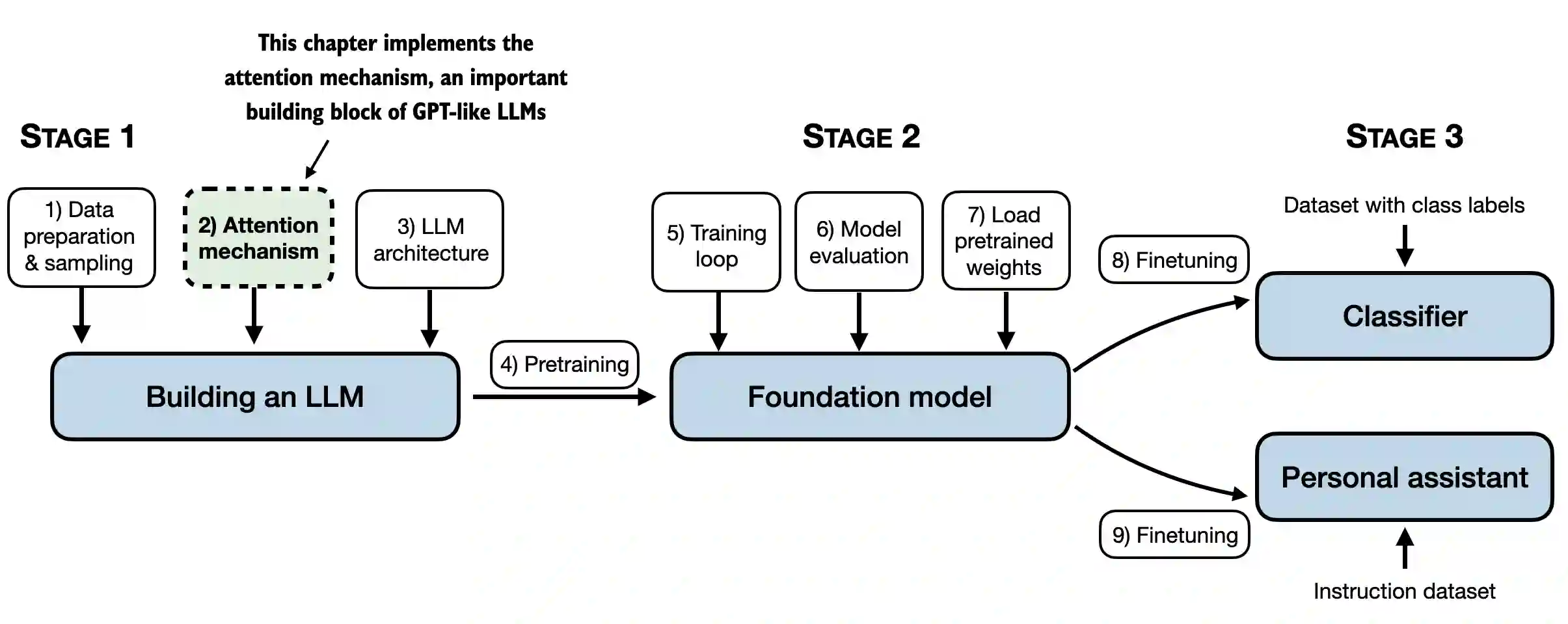
• 本章涵盖了注意力机制，LLM（大语言模型）的核心引擎。

3.1 模型长序列的问题

• 本节没有代码
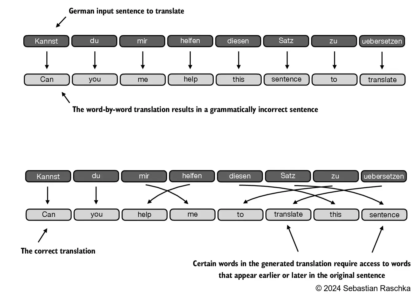
• 逐词翻译文本是不可行的，因为源语言和目标语言之间在语法结构上存在差异：

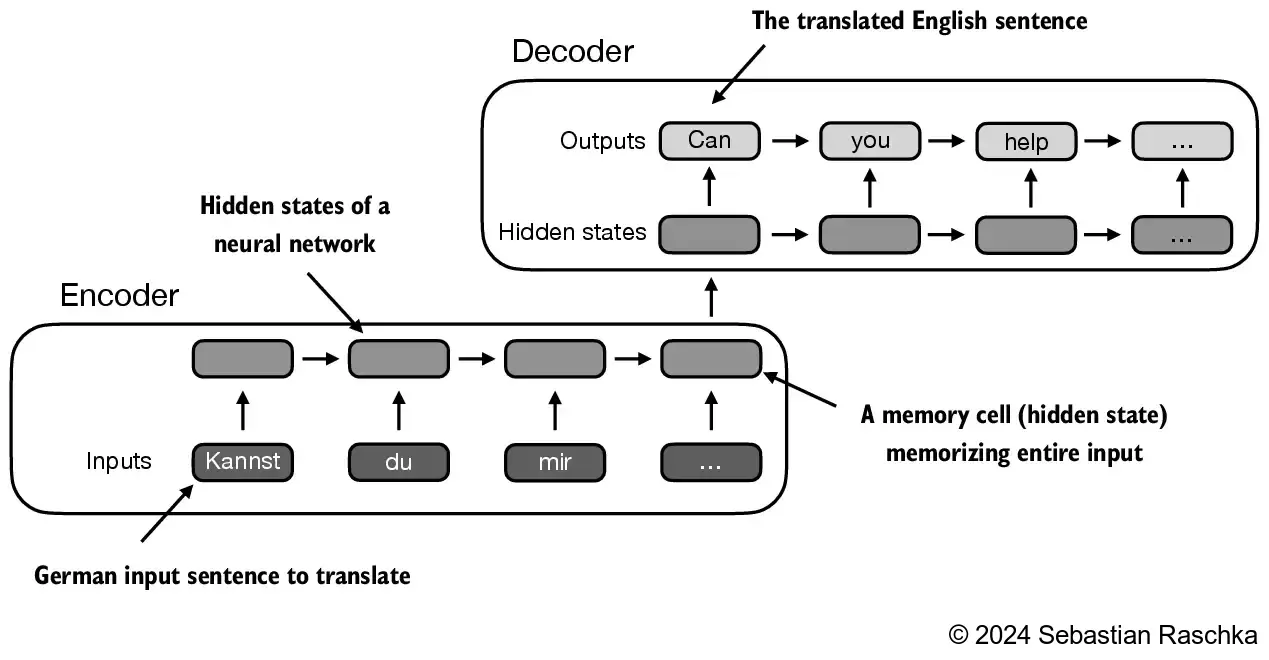
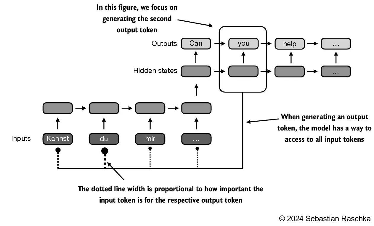
• 在引入 Transformer 模型之前，编码器-解码器 RNNs 被广泛用于机器翻译任务
• 在这种设置中，编码器处理来自源语言的标记序列，使用隐藏状态——一种神经网络内部的中间层——来生成整个输入序列的压缩表示：

3.2 捕获数据依赖关系的注意力机制

(Capturing data dependencies with attention mechanisms)

• 本节没有代码
• 通过注意力机制，文本生成解码器部分可以有选择地访问所有输入的tokens，这意味着某些输入tokens在生成特定输出token时比其他tokens更重要。

• Transformer中的自注意力（Self-attention）是一种技术，通过使序列中的每个位置能够与同一序列中的所有其他位置进行交互并确定它们的相关性，从而增强输入表示。

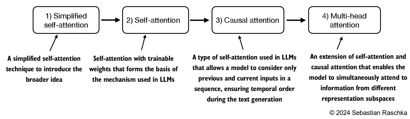
3.3 使用自注意力关注输入的不同部分

3.3.1 一个没有可训练权重的简单自注意力机制

• 本节解释了一个非常简化的自注意力变体，该变体不包含任何可训练的权重。
• 这个变体仅用于说明目的，并不是在变压器模型中使用的注意力机制。
• 下一节（第3.3.2节）将扩展这个简单的注意力机制，以实现真正的自注意力机制。
• 假设我们有一个输入序列 $x^{(1)}$ 到 $x^{(T)}$：
  • 输入是文本（例如一句话：“Your journey starts with one step”），已经按照第2章所描述的方式转化为令牌嵌入向量。
  • 比如，$x^{(1)}$ 是表示单词 “Your” 的一个 $d$ 维向量，依此类推。
• 目标：计算每个输入序列元素 $x^{(i)}$ 在 $x^{(1)}$ 到 $x^{(T)}$ 中的上下文向量 $z^{(i)}$（其中 $z$ 和 $x$ 具有相同的维度）。
  • 上下文向量 $z^{(i)}$ 是所有输入 $x^{(1)}$ 到 $x^{(T)}$ 的加权和。
  • 上下文向量是特定于某个输入的“上下文”。
    • 我们将不再把 $x^{(i)}$ 当作任意输入标记的占位符，而是考虑第二个输入 $x^{(2)}$。
    • 继续用一个具体的例子来说明，我们不再把 $z^{(i)}$ 当作占位符，而是考虑第二个输出上下文向量 $z^{(2)}$。
    • 第二个上下文向量 $z^{(2)}$ 是所有输入 $x^{(1)}$ 到 $x^{(T)}$ 的加权和，其中每个输入元素的权重与第二个输入元素 $x^{(2)}$ 相关。
    • 注意力权重就是在计算 $z^{(2)}$ 时，决定每个输入元素对加权和的贡献程度的权重。
    • 简而言之，可以把 $z^{(2)}$ 看作是 $x^{(2)}$ 的一个修改版本，它还结合了所有其他与当前任务相关的输入元素的信息。

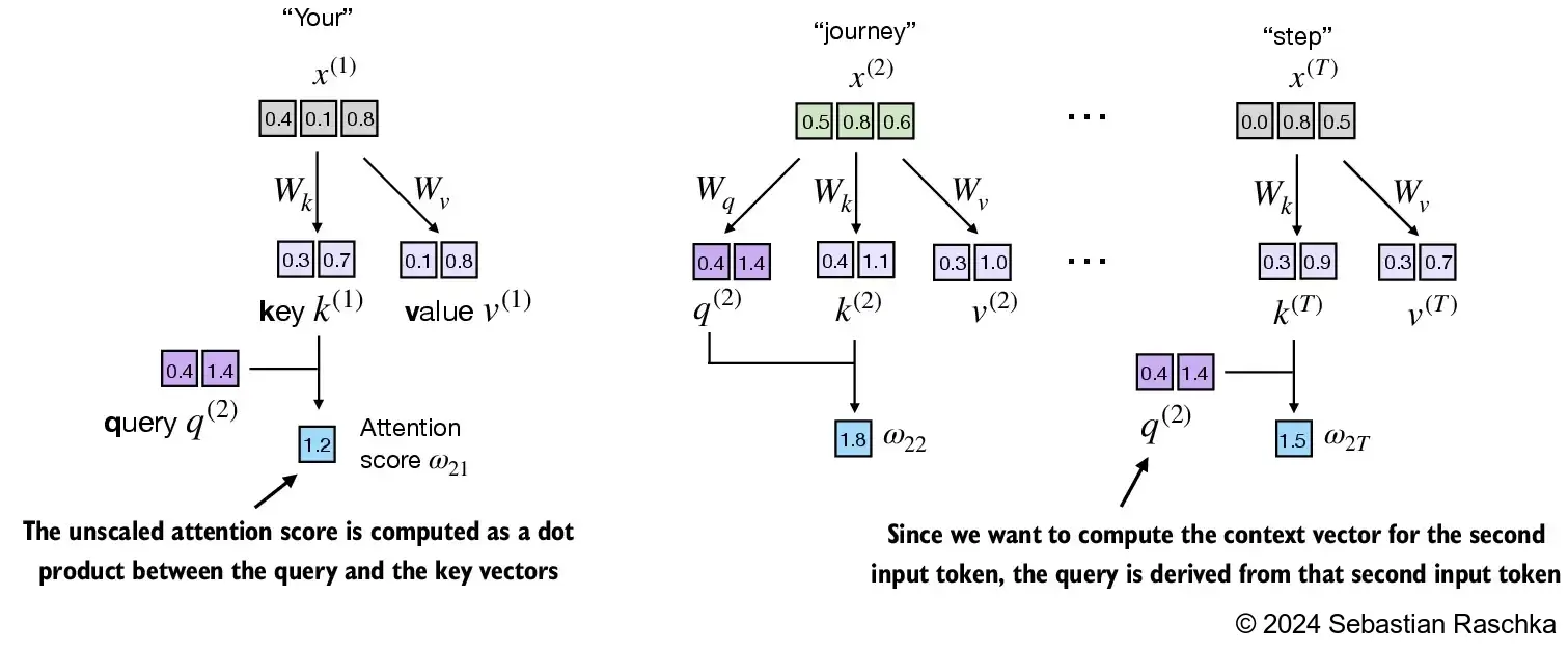
• （请注意，本图中的数字已截断为小数点后一个数字，以减少视觉干扰；类似地，其他图表中的数字也可能存在截断的情况）

• 按惯例，未归一化的注意力权重称为 “注意力得分”，而归一化后的注意力得分（其总和为1）称为 “注意力权重”

• 代码如下逐步演示了上面图示的计算过程

• 步骤 1: 计算未归一化的注意力得分 $\omega$

  • 假设我们使用第二个输入词元作为查询，即 $q^{(2)}=x^{(2)}$，通过点积计算未归一化的注意力得分：
    • ${\omega }_{21}=x^{(1)}{q}^{(2)\top }$
    • ${\omega }_{22}=x^{(2)}{q}^{(2)\top }$
    • ${\omega }_{23}=x^{(3)}{q}^{(2)\top }$
    • …
    • ${\omega }_{2T}=x^{(T)}{q}^{(2)\top }$

• 上述公式中的 $\omega$ 是希腊字母 “omega”，用来表示未归一化的注意力得分

  • 下标 “21” 表示输入序列元素 2 被用作查询，与输入序列元素 1 进行点积计算

• 假设我们有以下输入句子，它已经如第3章所述嵌入为3维向量（我们在这里使用非常小的嵌入维度，目的是为了便于展示，使其能在页面上显示而不产生换行）：

import torch

inputs = torch.tensor(
  [[0.43, 0.15, 0.89], # Your     (x^1)
   [0.55, 0.87, 0.66], # journey  (x^2)
   [0.57, 0.85, 0.64], # starts   (x^3)
   [0.22, 0.58, 0.33], # with     (x^4)
   [0.77, 0.25, 0.10], # one      (x^5)
   [0.05, 0.80, 0.55]] # step     (x^6)
)

• （在本书中，我们遵循常见的机器学习和深度学习惯例，其中训练样本表示为行，特征值表示为列；在上面显示的张量中，每一行代表一个单词，每一列代表一个嵌入维度）

• 本节的主要目标是演示如何使用第二个输入序列 $x^{(2)}$ 作为查询，计算上下文向量 $z^{(2)}$。

• 图示展示了这个过程的初步步骤，即通过点积运算计算 $x^{(2)}$ 和所有其他输入元素之间的注意力得分 $\omega$。

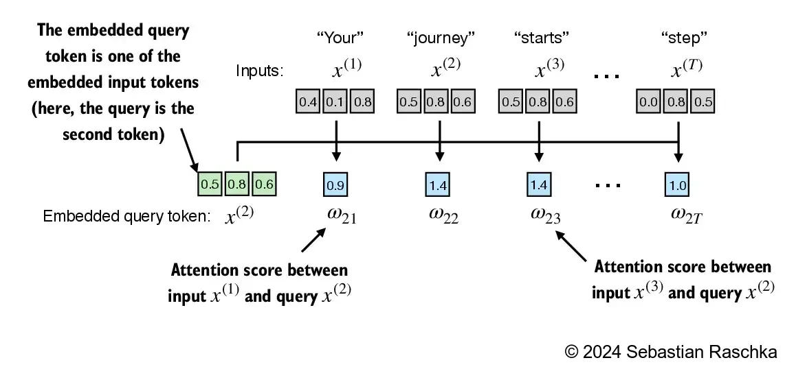
• 我们以输入序列元素 2，$x^{(2)}$，作为例子来计算上下文向量 $z^{(2)}$；在本节稍后，我们将对此进行推广，以计算所有上下文向量。
• 第一步是通过计算查询 $x^{(2)}$ 与所有其他输入标记的点积，来计算未归一化的注意力分数：

query = inputs[1]  # 2nd input token is the query

attn_scores_2 = torch.empty(inputs.shape[0])
for i, x_i in enumerate(inputs):
    attn_scores_2[i] = torch.dot(x_i, query) # dot product (transpose not necessary here since they are 1-dim vectors)

print(attn_scores_2)

tensor([0.9544, 1.4950, 1.4754, 0.8434, 0.7070, 1.0865])

• 附带说明：点积本质上是将两个向量按元素逐一相乘，并将结果相加的简写方式：

res = 0.

for idx, element in enumerate(inputs[0]):
    res += inputs[0][idx] * query[idx]

print(res)
print(torch.dot(inputs[0], query))

tensor(0.9544)
tensor(0.9544)

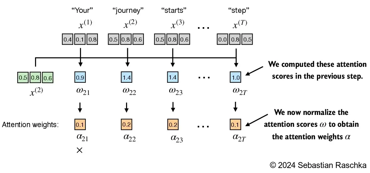
• 步骤 2： 将未归一化的注意力分数（“omegas”，$\omega$）归一化，使它们的和为 1。
• 这里有一种简单的方法将未归一化的注意力分数归一化，使它们的和为 1（这一约定有助于解释，并且对训练的稳定性非常重要）：

attn_weights_2_tmp = attn_scores_2 / attn_scores_2.sum()

print("Attention weights:", attn_weights_2_tmp)
print("Sum:", attn_weights_2_tmp.sum())

Attention weights: tensor([0.1455, 0.2278, 0.2249, 0.1285, 0.1077, 0.1656])
Sum: tensor(1.0000)

• 然而，在实践中，使用 softmax 函数进行归一化更为常见，因为它能更好地处理极端值，并且在训练过程中具有更理想的梯度属性，因此更为推荐。
• 下面是一个简单的 softmax 函数实现，用于缩放，它也会归一化向量元素，使它们的和为 1：

def softmax_naive(x):
    return torch.exp(x) / torch.exp(x).sum(dim=0)

attn_weights_2_naive = softmax_naive(attn_scores_2)

print("Attention weights:", attn_weights_2_naive)
print("Sum:", attn_weights_2_naive.sum())

Attention weights: tensor([0.1385, 0.2379, 0.2333, 0.1240, 0.1082, 0.1581])
Sum: tensor(1.)

• 上面的简单实现可能会由于溢出和下溢问题，在处理大或小输入值时出现数值不稳定的情况。
• 因此，在实践中，推荐使用 PyTorch 实现的 softmax 函数，因为它已经针对性能进行了高度优化：

attn_weights_2 = torch.softmax(attn_scores_2, dim=0)

print("Attention weights:", attn_weights_2)
print("Sum:", attn_weights_2.sum())

Attention weights: tensor([0.1385, 0.2379, 0.2333, 0.1240, 0.1082, 0.1581])
Sum: tensor(1.)

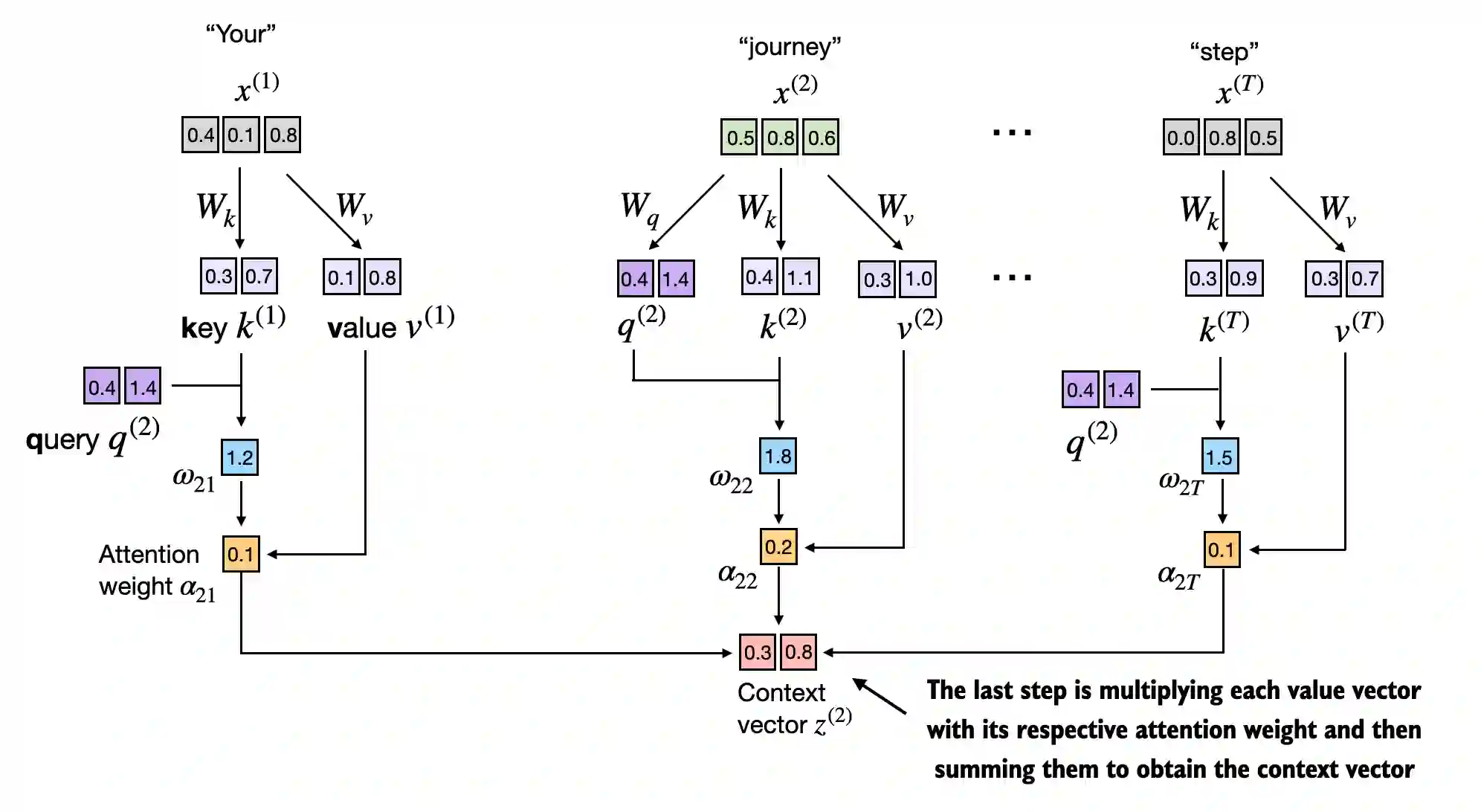
• 步骤 3：通过将嵌入的输入标记 $x^{(i)}$ 与注意力权重相乘，并将得到的向量求和，来计算上下文向量 $z^{(2)}$：

query = inputs[1] # 2nd input token is the query

context_vec_2 = torch.zeros(query.shape)
for i,x_i in enumerate(inputs):
    context_vec_2 += attn_weights_2[i]*x_i

print(context_vec_2)

tensor([0.4419, 0.6515, 0.5683])

3.3.2 计算所有输入标记的注意力权重

(Computing attention weights for all input tokens)

推广到所有输入序列的标记：

• 上面，我们计算了输入 2 的注意力权重和上下文向量（如下面图中高亮的行所示）。
• 接下来，我们将这个计算推广，计算所有输入标记的注意力权重和上下文向量。

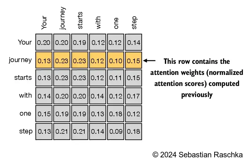
• （请注意，图中的数字被截断为小数点后两位，以减少视觉干扰；每一行的数值应该加起来为 1.0 或 100%；同样，其他图中的数字也经过了截断。）

• 在自注意力机制中，首先计算注意力分数，然后对其进行归一化，以得出总和为 1 的注意力权重。

• 然后，这些注意力权重被用来通过加权求和输入来生成上下文向量。

• 将之前的步骤 1应用于所有成对元素，计算未归一化的注意力分数矩阵：

attn_scores = torch.empty(6, 6)

for i, x_i in enumerate(inputs):
    for j, x_j in enumerate(inputs):
        attn_scores[i, j] = torch.dot(x_i, x_j)

print(attn_scores)

tensor([[0.9995, 0.9544, 0.9422, 0.4753, 0.4576, 0.6310],
        [0.9544, 1.4950, 1.4754, 0.8434, 0.7070, 1.0865],
        [0.9422, 1.4754, 1.4570, 0.8296, 0.7154, 1.0605],
        [0.4753, 0.8434, 0.8296, 0.4937, 0.3474, 0.6565],
        [0.4576, 0.7070, 0.7154, 0.3474, 0.6654, 0.2935],
        [0.6310, 1.0865, 1.0605, 0.6565, 0.2935, 0.9450]])

• 我们可以通过矩阵乘法更加高效地实现与上述相同的计算：

attn_scores = inputs @ inputs.T
print(attn_scores)

tensor([[0.9995, 0.9544, 0.9422, 0.4753, 0.4576, 0.6310],
        [0.9544, 1.4950, 1.4754, 0.8434, 0.7070, 1.0865],
        [0.9422, 1.4754, 1.4570, 0.8296, 0.7154, 1.0605],
        [0.4753, 0.8434, 0.8296, 0.4937, 0.3474, 0.6565],
        [0.4576, 0.7070, 0.7154, 0.3474, 0.6654, 0.2935],
        [0.6310, 1.0865, 1.0605, 0.6565, 0.2935, 0.9450]])

• 类似于之前的步骤 2，我们对每一行进行归一化处理，使得每一行的值加起来等于 1：

attn_weights = torch.softmax(attn_scores, dim=-1)
print(attn_weights)

tensor([[0.2098, 0.2006, 0.1981, 0.1242, 0.1220, 0.1452],
        [0.1385, 0.2379, 0.2333, 0.1240, 0.1082, 0.1581],
        [0.1390, 0.2369, 0.2326, 0.1242, 0.1108, 0.1565],
        [0.1435, 0.2074, 0.2046, 0.1462, 0.1263, 0.1720],
        [0.1526, 0.1958, 0.1975, 0.1367, 0.1879, 0.1295],
        [0.1385, 0.2184, 0.2128, 0.1420, 0.0988, 0.1896]])

• 快速验证每一行的值确实加起来等于 1：

row_2_sum = sum([0.1385, 0.2379, 0.2333, 0.1240, 0.1082, 0.1581])
print("Row 2 sum:", row_2_sum)

print("All row sums:", attn_weights.sum(dim=-1))

Row 2 sum: 1.0
All row sums: tensor([1.0000, 1.0000, 1.0000, 1.0000, 1.0000, 1.0000])

• 应用之前的步骤 3，计算所有的上下文向量：

all_context_vecs = attn_weights @ inputs
print(all_context_vecs)

tensor([[0.4421, 0.5931, 0.5790],
        [0.4419, 0.6515, 0.5683],
        [0.4431, 0.6496, 0.5671],
        [0.4304, 0.6298, 0.5510],
        [0.4671, 0.5910, 0.5266],
        [0.4177, 0.6503, 0.5645]])

• 作为合理性检查，之前计算的上下文向量 $z^{(2)}=[0.4419,0.6515,0.5683]$ 可以在上面计算结果的第二行找到：

print("Previous 2nd context vector:", context_vec_2)

Previous 2nd context vector: tensor([0.4419, 0.6515, 0.5683])

3.4 实现带有可训练权重的自注意力机制

(Implementing self-attention with trainable weights)

• 本节中开发的自注意力机制的概念框架，展示了它是如何融入本书和本章的整体叙事和结构中的。

3.4.1 逐步计算注意力权重

(Computing the attention weights step by step)

• 在本节中，我们将实现自注意力机制，这种机制被用于原始的 Transformer 架构、GPT 模型以及大多数其他流行的 LLM（大规模语言模型）中。
• 这种自注意力机制也被称为“缩放点积注意力”（scaled dot-product attention）。
• 总体思路与之前类似：
  • 我们希望计算上下文向量，通过对输入向量进行加权求和，针对特定的输入元素。
  • 为了实现这一点，我们需要计算注意力权重。
• 正如你将看到的，与之前介绍的基本注意力机制相比，差异非常小：
  • 最显著的区别是引入了在模型训练过程中会被更新的权重矩阵。
  • 这些可训练的权重矩阵非常关键，因为它们使得模型（特别是模型内部的注意力模块）能够学习如何生成“优良”的上下文向量。

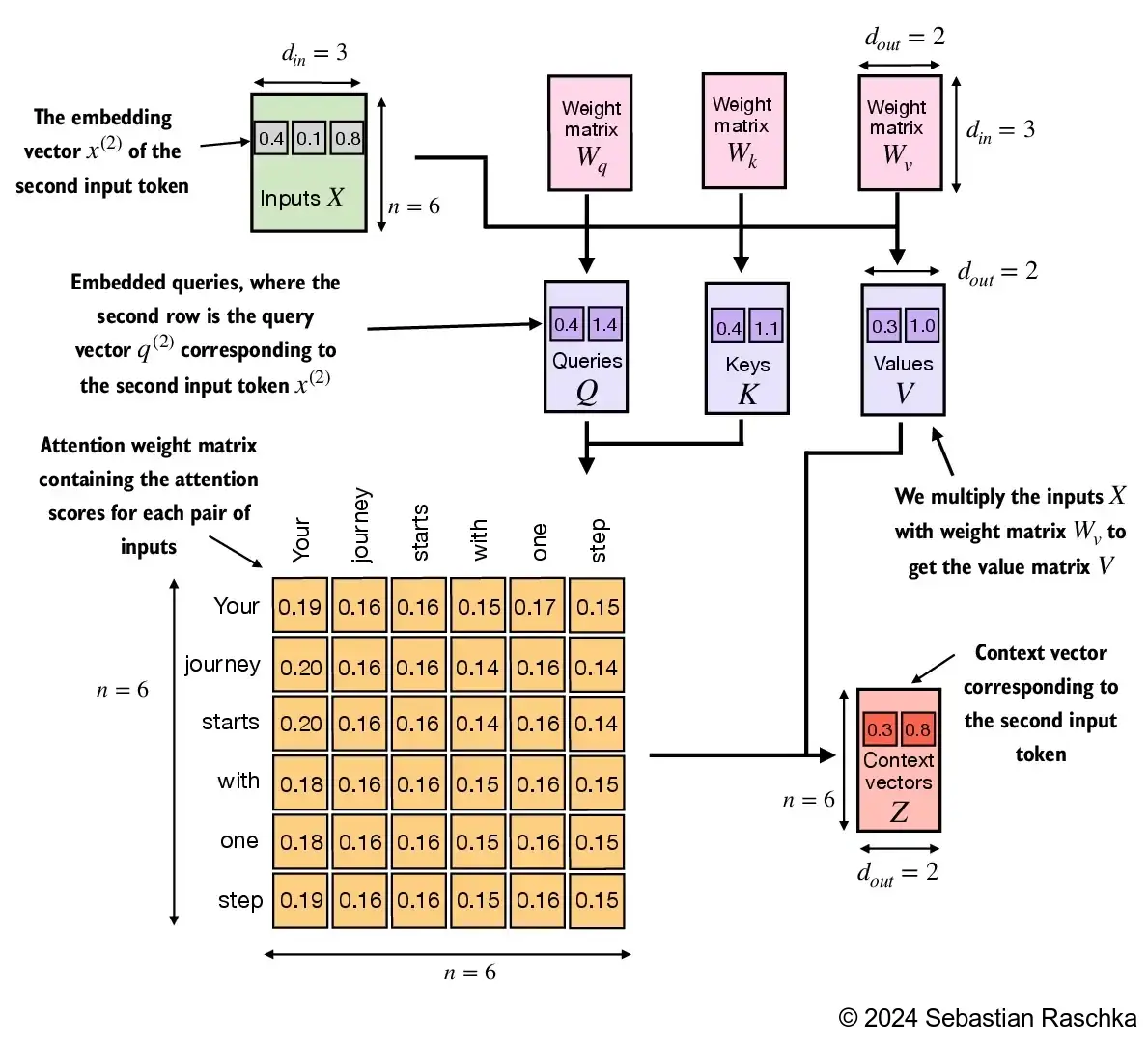
• 逐步实现自注意力机制，我们将首先引入三个训练权重矩阵 (W_q)、(W_k) 和 (W_v)。

• 这三个矩阵用于通过矩阵乘法将嵌入的输入标记 (x^{(i)}) 映射到查询、键和值向量：

  • 查询向量： (q^{(i)} = W_q , x^{(i)})
  • 键向量： (k^{(i)} = W_k , x^{(i)})
  • 值向量： (v^{(i)} = W_v , x^{(i)})

• 输入 (x) 和查询向量 (q) 的嵌入维度可以相同也可以不同，这取决于模型的设计和具体实现。

• 在 GPT 模型中，输入和输出的维度通常是相同的，但为了便于说明和更好地跟踪计算过程，这里我们选择不同的输入和输出维度：

x_2 = inputs[1] # second input element
d_in = inputs.shape[1] # the input embedding size, d=3
d_out = 2 # the output embedding size, d=2

• 以下，我们初始化这三个权重矩阵；请注意，我们将 requires_grad=False 设置为避免在输出中产生过多干扰，便于说明，但如果我们要使用这些权重矩阵进行模型训练，应该将 requires_grad=True，以便在训练过程中更新这些矩阵。

torch.manual_seed(123)

W_query = torch.nn.Parameter(torch.rand(d_in, d_out), requires_grad=False)
W_key   = torch.nn.Parameter(torch.rand(d_in, d_out), requires_grad=False)
W_value = torch.nn.Parameter(torch.rand(d_in, d_out), requires_grad=False)

• Next we compute the query, key, and value vectors:

query_2 = x_2 @ W_query # _2 because it's with respect to the 2nd input element
key_2 = x_2 @ W_key 
value_2 = x_2 @ W_value

print(query_2)

tensor([0.4306, 1.4551])

• 如下所示，我们成功地将 6 个输入标记从 3D 嵌入空间投影到 2D 嵌入空间：

keys = inputs @ W_key 
values = inputs @ W_value

print("keys.shape:", keys.shape)
print("values.shape:", values.shape)

keys.shape: torch.Size([6, 2])
values.shape: torch.Size([6, 2])

• 在下一步，步骤 2，我们通过计算查询向量与每个键向量的点积，来计算未归一化的注意力分数：

keys_2 = keys[1] # Python starts index at 0
attn_score_22 = query_2.dot(keys_2)
print(attn_score_22)

tensor(1.8524)

• 由于我们有 6 个输入，因此对于给定的查询向量，我们将得到 6 个注意力分数：

attn_scores_2 = query_2 @ keys.T # All attention scores for given query
print(attn_scores_2)

tensor([1.2705, 1.8524, 1.8111, 1.0795, 0.5577, 1.5440])

• 接下来，在步骤 3中，我们使用之前提到的 softmax 函数计算注意力权重（归一化的注意力分数，且其总和为 1）。
• 与之前的步骤不同的是，我们现在通过将注意力分数除以嵌入维度的平方根 (\sqrt{d_k})（即 d_k**0.5）来缩放注意力分数：

d_k = keys.shape[1]
attn_weights_2 = torch.softmax(attn_scores_2 / d_k**0.5, dim=-1)
print(attn_weights_2)

tensor([0.1500, 0.2264, 0.2199, 0.1311, 0.0906, 0.1820])

• 在步骤 4中，我们现在计算输入查询向量 2 的上下文向量：

context_vec_2 = attn_weights_2 @ values
print(context_vec_2)

tensor([0.3061, 0.8210])

3.4.2 实现一个简洁的 SelfAttention 类

(Implementing a compact SelfAttention class)

• 将所有步骤结合起来，我们可以如下实现自注意力机制：

import torch.nn as nn

class SelfAttention_v1(nn.Module):

    def __init__(self, d_in, d_out):
        super().__init__()
        self.W_query = nn.Parameter(torch.rand(d_in, d_out))
        self.W_key   = nn.Parameter(torch.rand(d_in, d_out))
        self.W_value = nn.Parameter(torch.rand(d_in, d_out))

    def forward(self, x):
        keys = x @ self.W_key
        queries = x @ self.W_query
        values = x @ self.W_value
        
        attn_scores = queries @ keys.T # omega
        attn_weights = torch.softmax(
            attn_scores / keys.shape[-1]**0.5, dim=-1
        )

        context_vec = attn_weights @ values
        return context_vec

torch.manual_seed(123)
sa_v1 = SelfAttention_v1(d_in, d_out)
print(sa_v1(inputs))

tensor([[0.2996, 0.8053],
        [0.3061, 0.8210],
        [0.3058, 0.8203],
        [0.2948, 0.7939],
        [0.2927, 0.7891],
        [0.2990, 0.8040]], grad_fn=<MmBackward0>)

• 我们可以使用 PyTorch 的 Linear 层来简化上面的实现，如果禁用偏置单元，它们相当于矩阵乘法。
• 使用 nn.Linear 相对于手动使用 nn.Parameter(torch.rand(...)) 的另一个重要优点是，nn.Linear 有一个推荐的权重初始化方案，这有助于模型训练的稳定性。

class SelfAttention_v2(nn.Module):

    def __init__(self, d_in, d_out, qkv_bias=False):
        super().__init__()
        self.W_query = nn.Linear(d_in, d_out, bias=qkv_bias)
        self.W_key   = nn.Linear(d_in, d_out, bias=qkv_bias)
        self.W_value = nn.Linear(d_in, d_out, bias=qkv_bias)

    def forward(self, x):
        keys = self.W_key(x)
        queries = self.W_query(x)
        values = self.W_value(x)
        
        attn_scores = queries @ keys.T
        attn_weights = torch.softmax(attn_scores / keys.shape[-1]**0.5, dim=-1)

        context_vec = attn_weights @ values
        return context_vec

torch.manual_seed(789)
sa_v2 = SelfAttention_v2(d_in, d_out)
print(sa_v2(inputs))

tensor([[-0.0739,  0.0713],
        [-0.0748,  0.0703],
        [-0.0749,  0.0702],
        [-0.0760,  0.0685],
        [-0.0763,  0.0679],
        [-0.0754,  0.0693]], grad_fn=<MmBackward0>)

• 请注意，SelfAttention_v1 和 SelfAttention_v2 给出的输出是不同的，因为它们使用了不同的初始权重矩阵。

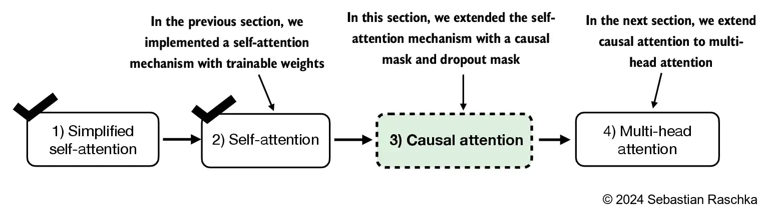
3.5 通过因果注意力隐藏未来的词汇

(Hiding future words with causal attention)

• 在因果注意力中，对角线以上的注意力权重会被屏蔽，确保对于任何给定的输入，LLM 在计算上下文向量时无法使用未来的标记。

3.5.1 应用因果注意力掩码

(Applying a causal attention mask)

• 在本节中，我们将之前的自注意力机制转换为因果自注意力机制。
• 因果自注意力确保模型在预测序列中某个位置的值时，只依赖于前面位置的已知输出，而不依赖于未来的位置。
• 简而言之，这确保了每个下一个单词的预测仅应依赖于前面的单词。
• 为了实现这一点，对于每个给定的标记，我们会屏蔽掉未来的标记（即在输入文本中当前标记之后的标记）：

• 为了说明和实现因果自注意力，我们将使用上一节中的注意力分数和权重：

# Reuse the query and key weight matrices of the
# SelfAttention_v2 object from the previous section for convenience
queries = sa_v2.W_query(inputs)
keys = sa_v2.W_key(inputs) 
attn_scores = queries @ keys.T

attn_weights = torch.softmax(attn_scores / keys.shape[-1]**0.5, dim=-1)
print(attn_weights)

tensor([[0.1921, 0.1646, 0.1652, 0.1550, 0.1721, 0.1510],
        [0.2041, 0.1659, 0.1662, 0.1496, 0.1665, 0.1477],
        [0.2036, 0.1659, 0.1662, 0.1498, 0.1664, 0.1480],
        [0.1869, 0.1667, 0.1668, 0.1571, 0.1661, 0.1564],
        [0.1830, 0.1669, 0.1670, 0.1588, 0.1658, 0.1585],
        [0.1935, 0.1663, 0.1666, 0.1542, 0.1666, 0.1529]],
       grad_fn=<SoftmaxBackward0>)

• 屏蔽未来注意力权重的最简单方法是通过使用 PyTorch 的 tril 函数创建一个掩码，将主对角线以下的元素（包括对角线本身）设置为 1，将主对角线以上的元素设置为 0：

context_length = attn_scores.shape[0]
mask_simple = torch.tril(torch.ones(context_length, context_length))
print(mask_simple)

tensor([[1., 0., 0., 0., 0., 0.],
        [1., 1., 0., 0., 0., 0.],
        [1., 1., 1., 0., 0., 0.],
        [1., 1., 1., 1., 0., 0.],
        [1., 1., 1., 1., 1., 0.],
        [1., 1., 1., 1., 1., 1.]])

• 然后，我们可以将注意力权重与这个掩码相乘，将对角线以上的注意力分数置为零：

masked_simple = attn_weights*mask_simple
print(masked_simple)

tensor([[0.1921, 0.0000, 0.0000, 0.0000, 0.0000, 0.0000],
        [0.2041, 0.1659, 0.0000, 0.0000, 0.0000, 0.0000],
        [0.2036, 0.1659, 0.1662, 0.0000, 0.0000, 0.0000],
        [0.1869, 0.1667, 0.1668, 0.1571, 0.0000, 0.0000],
        [0.1830, 0.1669, 0.1670, 0.1588, 0.1658, 0.0000],
        [0.1935, 0.1663, 0.1666, 0.1542, 0.1666, 0.1529]],
       grad_fn=<MulBackward0>)

• 然而，如果掩码在 softmax 之后应用，就像上面那样，它会破坏由 softmax 创建的概率分布。

• Softmax 确保所有输出值的和为 1。

• 在 softmax 之后应用掩码需要重新归一化输出，使其和为 1，这会使过程变得复杂，并可能导致一些意外的效果。

• 为了确保每一行的和为 1，我们可以按如下方式对注意力权重进行归一化：

row_sums = masked_simple.sum(dim=-1, keepdim=True)
masked_simple_norm = masked_simple / row_sums
print(masked_simple_norm)

tensor([[1.0000, 0.0000, 0.0000, 0.0000, 0.0000, 0.0000],
        [0.5517, 0.4483, 0.0000, 0.0000, 0.0000, 0.0000],
        [0.3800, 0.3097, 0.3103, 0.0000, 0.0000, 0.0000],
        [0.2758, 0.2460, 0.2462, 0.2319, 0.0000, 0.0000],
        [0.2175, 0.1983, 0.1984, 0.1888, 0.1971, 0.0000],
        [0.1935, 0.1663, 0.1666, 0.1542, 0.1666, 0.1529]],
       grad_fn=<DivBackward0>)

• 虽然我们现在从技术上讲已经完成了因果注意力机制的编码，但我们还是简单看一下一个更高效的方法来实现与上述相同的效果。
• 因此，我们可以在注意力分数进入 softmax 函数之前，将对角线以上的未归一化的注意力分数用负无穷大进行屏蔽，而不是将注意力权重置为零并重新归一化结果：

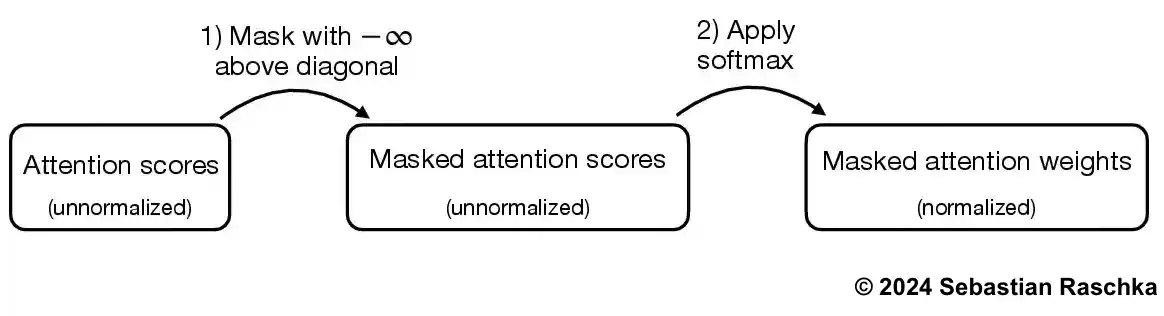
mask = torch.triu(torch.ones(context_length, context_length), diagonal=1)
masked = attn_scores.masked_fill(mask.bool(), -torch.inf)
print(masked)

tensor([[0.2899,   -inf,   -inf,   -inf,   -inf,   -inf],
        [0.4656, 0.1723,   -inf,   -inf,   -inf,   -inf],
        [0.4594, 0.1703, 0.1731,   -inf,   -inf,   -inf],
        [0.2642, 0.1024, 0.1036, 0.0186,   -inf,   -inf],
        [0.2183, 0.0874, 0.0882, 0.0177, 0.0786,   -inf],
        [0.3408, 0.1270, 0.1290, 0.0198, 0.1290, 0.0078]],
       grad_fn=<MaskedFillBackward0>)

• 如下所示，现在每一行的注意力权重正确地重新归一化，和为 1：

attn_weights = torch.softmax(masked / keys.shape[-1]**0.5, dim=-1)
print(attn_weights)

tensor([[1.0000, 0.0000, 0.0000, 0.0000, 0.0000, 0.0000],
        [0.5517, 0.4483, 0.0000, 0.0000, 0.0000, 0.0000],
        [0.3800, 0.3097, 0.3103, 0.0000, 0.0000, 0.0000],
        [0.2758, 0.2460, 0.2462, 0.2319, 0.0000, 0.0000],
        [0.2175, 0.1983, 0.1984, 0.1888, 0.1971, 0.0000],
        [0.1935, 0.1663, 0.1666, 0.1542, 0.1666, 0.1529]],
       grad_fn=<SoftmaxBackward0>)

3.5.2 使用 Dropout 屏蔽额外的注意力权重

(Masking additional attention weights with dropout)

• 此外，我们还应用了 dropout 来减少训练过程中的过拟合。

• Dropout 可以应用在多个地方：

  • 例如，在计算注意力权重后；
  • 或者在将注意力权重与值向量相乘后。

• 在这里，我们将在计算注意力权重后应用 dropout 掩码，因为这种方式更为常见。

• 此外，在这个具体的例子中，我们使用了 50% 的 dropout 率，这意味着我们随机屏蔽一半的注意力权重。（当我们稍后训练 GPT 模型时，我们会使用更低的 dropout 率，比如 0.1 或 0.2）

• 如果我们应用 0.5（50%）的 dropout 率，那么未被屏蔽的值将按比例放大，放大因子为 1 / 0.5 = 2。
• 这个缩放因子是通过公式 1 / (1 - dropout_rate) 计算的。

torch.manual_seed(123)
dropout = torch.nn.Dropout(0.5) # dropout rate of 50%
example = torch.ones(6, 6) # create a matrix of ones

print(dropout(example))

tensor([[2., 2., 0., 2., 2., 0.],
        [0., 0., 0., 2., 0., 2.],
        [2., 2., 2., 2., 0., 2.],
        [0., 2., 2., 0., 0., 2.],
        [0., 2., 0., 2., 0., 2.],
        [0., 2., 2., 2., 2., 0.]])

torch.manual_seed(123)
print(dropout(attn_weights))

tensor([[2.0000, 0.0000, 0.0000, 0.0000, 0.0000, 0.0000],
        [0.0000, 0.0000, 0.0000, 0.0000, 0.0000, 0.0000],
        [0.7599, 0.6194, 0.6206, 0.0000, 0.0000, 0.0000],
        [0.0000, 0.4921, 0.4925, 0.0000, 0.0000, 0.0000],
        [0.0000, 0.3966, 0.0000, 0.3775, 0.0000, 0.0000],
        [0.0000, 0.3327, 0.3331, 0.3084, 0.3331, 0.0000]],
       grad_fn=<MulBackward0>)

• 请注意，结果的 dropout 输出可能会根据操作系统的不同而有所不同；你可以在 PyTorch 问题跟踪器 上阅读更多关于这种不一致性的内容。

3.5.3 实现一个简洁的因果自注意力类

(Implementing a compact causal self-attention class)

• 现在，我们准备实现一个完整的自注意力机制，包括因果屏蔽和 dropout 屏蔽。
• 另一个需要实现的部分是处理包含多个输入的批处理，以便我们的 CausalAttention 类能够支持由第二章中实现的数据加载器生成的批处理输出。
• 为了简化，模拟这种批处理输入，我们将输入文本示例复制多次：

batch = torch.stack((inputs, inputs), dim=0)
print(batch.shape) # 2 inputs with 6 tokens each, and each token has embedding dimension 3

torch.Size([2, 6, 3])

class CausalAttention(nn.Module):

    def __init__(self, d_in, d_out, context_length,
                 dropout, qkv_bias=False):
        super().__init__()
        self.d_out = d_out
        self.W_query = nn.Linear(d_in, d_out, bias=qkv_bias)
        self.W_key   = nn.Linear(d_in, d_out, bias=qkv_bias)
        self.W_value = nn.Linear(d_in, d_out, bias=qkv_bias)
        self.dropout = nn.Dropout(dropout) # New
        self.register_buffer('mask', torch.triu(torch.ones(context_length, context_length), diagonal=1)) # New

    def forward(self, x):
        b, num_tokens, d_in = x.shape # New batch dimension b
        keys = self.W_key(x)
        queries = self.W_query(x)
        values = self.W_value(x)

        attn_scores = queries @ keys.transpose(1, 2) # Changed transpose
        attn_scores.masked_fill_(  # New, _ ops are in-place
            self.mask.bool()[:num_tokens, :num_tokens], -torch.inf)  # `:num_tokens` to account for cases where the number of tokens in the batch is smaller than the supported context_size
        attn_weights = torch.softmax(
            attn_scores / keys.shape[-1]**0.5, dim=-1
        )
        attn_weights = self.dropout(attn_weights) # New

        context_vec = attn_weights @ values
        return context_vec

torch.manual_seed(123)

context_length = batch.shape[1]
ca = CausalAttention(d_in, d_out, context_length, 0.0)

context_vecs = ca(batch)

print(context_vecs)
print("context_vecs.shape:", context_vecs.shape)

tensor([[[-0.4519,  0.2216],
         [-0.5874,  0.0058],
         [-0.6300, -0.0632],
         [-0.5675, -0.0843],
         [-0.5526, -0.0981],
         [-0.5299, -0.1081]],

        [[-0.4519,  0.2216],
         [-0.5874,  0.0058],
         [-0.6300, -0.0632],
         [-0.5675, -0.0843],
         [-0.5526, -0.0981],
         [-0.5299, -0.1081]]], grad_fn=<UnsafeViewBackward0>)
context_vecs.shape: torch.Size([2, 6, 2])

• 请注意，dropout 只在训练期间应用，而在推理期间不应用。

3.6 将单头注意力扩展到多头注意力

(Extending single-head attention to multi-head attention)

3.6.1 堆叠多个单头注意力层

• 以下是之前实现的自注意力的总结（为了简便，未显示因果和 dropout 掩码）

• 这也被称为单头注意力：

• 我们只需将多个单头注意力模块堆叠在一起，就可以得到一个多头注意力模块：

• 多头注意力背后的主要思想是多次（并行地）运行注意力机制，每次使用不同的、学习到的线性投影。这使得模型能够在不同的位置同时关注来自不同表示子空间的信息。

class MultiHeadAttentionWrapper(nn.Module):

    def __init__(self, d_in, d_out, context_length, dropout, num_heads, qkv_bias=False):
        super().__init__()
        self.heads = nn.ModuleList(
            [CausalAttention(d_in, d_out, context_length, dropout, qkv_bias) 
             for _ in range(num_heads)]
        )

    def forward(self, x):
        return torch.cat([head(x) for head in self.heads], dim=-1)


torch.manual_seed(123)

context_length = batch.shape[1] # This is the number of tokens
d_in, d_out = 3, 2
mha = MultiHeadAttentionWrapper(
    d_in, d_out, context_length, 0.0, num_heads=2
)

context_vecs = mha(batch)

print(context_vecs)
print("context_vecs.shape:", context_vecs.shape)

tensor([[[-0.4519,  0.2216,  0.4772,  0.1063],
         [-0.5874,  0.0058,  0.5891,  0.3257],
         [-0.6300, -0.0632,  0.6202,  0.3860],
         [-0.5675, -0.0843,  0.5478,  0.3589],
         [-0.5526, -0.0981,  0.5321,  0.3428],
         [-0.5299, -0.1081,  0.5077,  0.3493]],

        [[-0.4519,  0.2216,  0.4772,  0.1063],
         [-0.5874,  0.0058,  0.5891,  0.3257],
         [-0.6300, -0.0632,  0.6202,  0.3860],
         [-0.5675, -0.0843,  0.5478,  0.3589],
         [-0.5526, -0.0981,  0.5321,  0.3428],
         [-0.5299, -0.1081,  0.5077,  0.3493]]], grad_fn=<CatBackward0>)
context_vecs.shape: torch.Size([2, 6, 4])

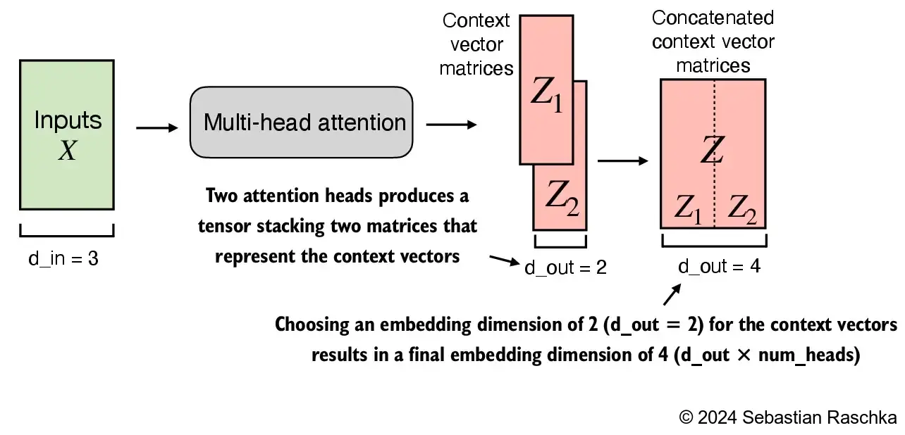
• 在上述实现中，嵌入维度为 4，因为我们将 d_out=2 作为键、查询和值向量以及上下文向量的嵌入维度。由于我们有 2 个注意力头，因此输出嵌入维度为 2 * 2 = 4。

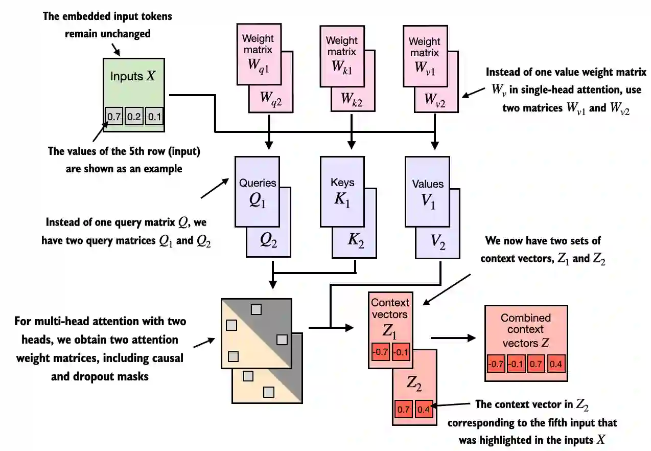
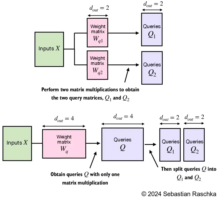
3.6.2 实现带有权重拆分的多头注意力

• 虽然上述实现是一个直观且完全可行的多头注意力实现（将之前的单头注意力 CausalAttention 实现进行了封装），我们可以编写一个独立的类叫做 MultiHeadAttention 来实现相同的功能。

• 对于这个独立的 MultiHeadAttention 类，我们不需要将单个注意力头进行拼接。

• 相反，我们创建单独的 W_query、W_key 和 W_value 权重矩阵，然后将这些矩阵拆分成每个注意力头的独立矩阵：

class MultiHeadAttention(nn.Module):
    def __init__(self, d_in, d_out, context_length, dropout, num_heads, qkv_bias=False):
        super().__init__()
        assert (d_out % num_heads == 0), \
            "d_out must be divisible by num_heads"

        self.d_out = d_out
        self.num_heads = num_heads
        self.head_dim = d_out // num_heads # Reduce the projection dim to match desired output dim

        self.W_query = nn.Linear(d_in, d_out, bias=qkv_bias)
        self.W_key = nn.Linear(d_in, d_out, bias=qkv_bias)
        self.W_value = nn.Linear(d_in, d_out, bias=qkv_bias)
        self.out_proj = nn.Linear(d_out, d_out)  # Linear layer to combine head outputs
        self.dropout = nn.Dropout(dropout)
        self.register_buffer(
            "mask",
            torch.triu(torch.ones(context_length, context_length),
                       diagonal=1)
        )

    def forward(self, x):
        b, num_tokens, d_in = x.shape

        keys = self.W_key(x) # Shape: (b, num_tokens, d_out)
        queries = self.W_query(x)
        values = self.W_value(x)

        # We implicitly split the matrix by adding a `num_heads` dimension
        # Unroll last dim: (b, num_tokens, d_out) -> (b, num_tokens, num_heads, head_dim)
        keys = keys.view(b, num_tokens, self.num_heads, self.head_dim) 
        values = values.view(b, num_tokens, self.num_heads, self.head_dim)
        queries = queries.view(b, num_tokens, self.num_heads, self.head_dim)

        # Transpose: (b, num_tokens, num_heads, head_dim) -> (b, num_heads, num_tokens, head_dim)
        keys = keys.transpose(1, 2)
        queries = queries.transpose(1, 2)
        values = values.transpose(1, 2)

        # Compute scaled dot-product attention (aka self-attention) with a causal mask
        attn_scores = queries @ keys.transpose(2, 3)  # Dot product for each head

        # Original mask truncated to the number of tokens and converted to boolean
        mask_bool = self.mask.bool()[:num_tokens, :num_tokens]

        # Use the mask to fill attention scores
        attn_scores.masked_fill_(mask_bool, -torch.inf)
        
        attn_weights = torch.softmax(attn_scores / keys.shape[-1]**0.5, dim=-1)
        attn_weights = self.dropout(attn_weights)

        # Shape: (b, num_tokens, num_heads, head_dim)
        context_vec = (attn_weights @ values).transpose(1, 2) 
        
        # Combine heads, where self.d_out = self.num_heads * self.head_dim
        context_vec = context_vec.contiguous().view(b, num_tokens, self.d_out)
        context_vec = self.out_proj(context_vec) # optional projection

        return context_vec

torch.manual_seed(123)

batch_size, context_length, d_in = batch.shape
d_out = 2
mha = MultiHeadAttention(d_in, d_out, context_length, 0.0, num_heads=2)

context_vecs = mha(batch)

print(context_vecs)
print("context_vecs.shape:", context_vecs.shape)

tensor([[[0.3190, 0.4858],
         [0.2943, 0.3897],
         [0.2856, 0.3593],
         [0.2693, 0.3873],
         [0.2639, 0.3928],
         [0.2575, 0.4028]],

        [[0.3190, 0.4858],
         [0.2943, 0.3897],
         [0.2856, 0.3593],
         [0.2693, 0.3873],
         [0.2639, 0.3928],
         [0.2575, 0.4028]]], grad_fn=<ViewBackward0>)
context_vecs.shape: torch.Size([2, 6, 2])

• 请注意，上述实现本质上是 MultiHeadAttentionWrapper 的重写版本，且更加高效。
• 由于随机权重初始化不同，最终的输出看起来有些不同，但两者都是完全可行的实现，可以在我们接下来章节中实现的 GPT 类中使用。
• 另外，注意我们在上述的 MultiHeadAttention 类中添加了一个线性投影层（self.out_proj）。这仅仅是一个线性变换，不会改变维度。在 LLM 实现中，使用这样的投影层是标准惯例，但并不是严格必要的（最近的研究表明，在不影响模型性能的情况下可以去除该层；有关更多信息，请参见本章末尾的进一步阅读部分）。

• 请注意，如果你对上述内容的紧凑且高效的实现感兴趣，你还可以考虑使用 PyTorch 中的 torch.nn.MultiheadAttention 类。

• 由于上述实现初看起来可能有些复杂，我们来看看执行 attn_scores = queries @ keys.transpose(2, 3) 时发生了什么：

# (b, num_heads, num_tokens, head_dim) = (1, 2, 3, 4)
a = torch.tensor([[[[0.2745, 0.6584, 0.2775, 0.8573],
                    [0.8993, 0.0390, 0.9268, 0.7388],
                    [0.7179, 0.7058, 0.9156, 0.4340]],

                   [[0.0772, 0.3565, 0.1479, 0.5331],
                    [0.4066, 0.2318, 0.4545, 0.9737],
                    [0.4606, 0.5159, 0.4220, 0.5786]]]])

print(a @ a.transpose(2, 3))

tensor([[[[1.3208, 1.1631, 1.2879],
          [1.1631, 2.2150, 1.8424],
          [1.2879, 1.8424, 2.0402]],

         [[0.4391, 0.7003, 0.5903],
          [0.7003, 1.3737, 1.0620],
          [0.5903, 1.0620, 0.9912]]]])

• 在这种情况下，PyTorch 中的矩阵乘法实现将处理 4 维输入张量，使得矩阵乘法在最后两个维度（num_tokens, head_dim）之间进行，然后对每个注意力头分别执行。

• 例如，以下是计算每个头的矩阵乘法的更简洁方式：

first_head = a[0, 0, :, :]
first_res = first_head @ first_head.T
print("First head:\n", first_res)

second_head = a[0, 1, :, :]
second_res = second_head @ second_head.T
print("\nSecond head:\n", second_res)

First head:
 tensor([[1.3208, 1.1631, 1.2879],
        [1.1631, 2.2150, 1.8424],
        [1.2879, 1.8424, 2.0402]])

Second head:
 tensor([[0.4391, 0.7003, 0.5903],
        [0.7003, 1.3737, 1.0620],
        [0.5903, 1.0620, 0.9912]])