
教科书:MATLAB语音信号分析与合成(第2版)
链接(含配套源代码):https://pan.baidu.com/s/1pXMPD_9TRpJmubPGaRKANw?pwd=32rf
提取码:32rf
基础入门视频:
视频链接:
配套练习:
任务:利用线性预测模型,寻找 汉语韵母 的共振峰
• 第 1 步:在安静的环境中,(建议用手机)录制声音
• 发音内容: a 、 e 、 i 、 o 、 u (“阿、婀、依、哦、乌”)
• 建议发音时尽量平稳、清晰
• 第 2 步:将一整段声音分为多帧,对每一帧 𝑥[𝑛] 进行 分析
• 使用 MATLAB 提供的 lpc 函数(或 levinson 函数),得到每一帧的
线性预测系数 𝑎 1 , ⋯ , 𝑎 𝑃 ,进而可得该帧的激励信号 𝑒[𝑛]
• 第 3 步:找到滤波器 1/𝐴(𝑧) 幅度谱的前两个共振峰频率值 𝑓 1 和 𝑓 2
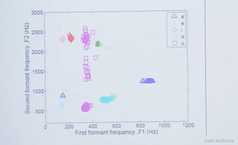
• 第 4 步:画出每个韵母的共振峰频率值 𝑓 2 vs 𝑓 1 (横轴为 𝑓 1 ,纵轴为 𝑓 2 )
实验结果参考:
参考代码(需要对这个代码进行修改才能完成任务,这个代码也是清华老师刘奕汶给学生做这个实验提供的代码):
%% DSP_lab5_2024_LP_demo_rb_v0_1.m
% For the course EEG3024B: DSP Technology and Its Applications at Shantou University
% ZHANG Rongbin,  20 Apr 2024

% Adapted based on ASAS_lab6_LinPred_2015.m by Prof. Yi-Wen Liu
% EE6641 HW: Linear prediction and Levinson-Durbin k-parameter estimation
% Created May 2013 as a homework.
% Last updated Nov 2015 for this year's Lab6 and HW3.
% Yi-Wen Liu


clear;
close all;

DIR = './';

FILENAME = 'a1.mp3';
% FILENAME = 'i1.mp3';

[y, fs1] = audioread([DIR FILENAME]);
y = y(:, 1);  % Obtain the first channel in case the audio file has multiple channels
% figure; plot(y);

y = y(60000 : end - 60000);
% figure; plot(y);

soundsc(y, fs1);
fs = 16000;  % sampling frequency, in Hz

y = resample(y, fs, fs1);

%% Parameters to play with
framelen = 0.04; % Frame length, in second. Please try changing this.
p = 16; % linear prediction order. Please try changing this.

%%
L = framelen*fs; % Frame length, in samples

if L <= p
    disp('Linear prediction requires the num of equations to be greater than the number of variables.');
end

sw.emphasis = 1; % default = 1  (Used to pre-emphasis the high frequency components)

numFrames = floor(length(y)/L);
excitat = zeros(size(y));   % excitation signal
e_n = zeros(p+L,1);

LPcoeffs = zeros(p+1,numFrames);
Kcoeffs = zeros(p,numFrames); % reflection coeffs

Nfreqs = 1024; % Num points for plotting the inverse filter response
df = fs/2/Nfreqs;
ff = 0:df:fs/2-df;

if sw.emphasis == 1
    y_emph = filter([1 -0.95],1,y);
else
    y_emph = y;
end

h = figure;
h_pos = h.Position;
set(h, 'Position', [0.5*h_pos(1)   0.5*h_pos(2)   h_pos(3)*1.3   h_pos(4)*1.3]);

%% Linear prediction and estimation of the source e_n
win = ones(L,1); % Rectangular window.
lpc_1_levinson_0 = 0;   % Indicator, 1 for using lpc() function, 0 for using levinson() function
for kk = 1:numFrames
    ind = (kk-1)*L+1 : kk*L;
    ywin = y_emph(ind).*win;
    Y = fft(ywin, 2^nextpow2(2*size(ywin,1)-1));
% 	Y = fft(ywin, Nfreqs*2);

    if lpc_1_levinson_0 == 1
        %% Use MATLAB's lpc() function
        A = lpc(ywin, p); %% This is actually the direct way to obtain the LP coefficients.
    else
        %% Or, use Levinson-Durbin algorithm
        % We can used levinson() instead because it gives us the "reflection coefficients".
        R = ifft(abs(Y).^2);
        [A, errvar, K] = levinson(R, p);
    end

    if kk == 1
        e_n(p+1 : end) = filter(A, [1], ywin);
    else
        ywin_extended = y((kk-1)*L+1-p : kk*L);
        e_n = filter(A, [1], ywin_extended);
    end
    excitat(ind) = e_n(p+1 : end);

    if kk>1
        subplot(311);
        plot(ind/fs*1000, y(ind), 'b', 'LineWidth', 1.5);
        xlabel('Time (in ms)', 'Interpreter', 'latex', 'fontSize', 14);
        ylabel('$x(n)$', 'Interpreter', 'latex', 'fontSize',14);
        title('Time Domain: $x(n)$', 'Interpreter', 'latex', 'fontSize', 16);
        set(gca, 'xlim', [kk-1 kk]*framelen*1000);
        grid on;    ax = gca;         ax.GridLineStyle = '--';        grid minor;

        subplot(312);
        plot(ind/fs*1000, e_n(p+1:end), 'k', 'LineWidth', 1.5);
        xlabel('Time (in ms)', 'Interpreter', 'latex', 'fontSize', 14);
        ylabel('$e(n)$', 'Interpreter', 'latex', 'fontSize', 14);
        title('Time Domain: $e(n)$', 'Interpreter', 'latex', 'fontSize', 16);
        set(gca, 'xlim', [kk-1 kk]*framelen*1000);
        grid on;    ax = gca;         ax.GridLineStyle = '--';        grid minor;

        subplot(313);
        [H, W] = freqz(1, A, Nfreqs);
        Hmag = 20*log10(abs(H));
        Ymag = 20*log10(abs(Y(1:Nfreqs)));
        Hmax = max(Hmag);
        offset = max(Hmag) - max(Ymag);
        plot(ff, Ymag+offset, 'b', 'LineWidth', 1); hold on;
        plot(ff, Hmag, 'r', 'LineWidth', 3); hold off;
        if kk == numFrames
            legend('$|X(\omega)|$ of $x(n)$', '$|A(\omega)|$ of LPC $\{ a_k \}$', ...
                'Location', 'NorthEast', 'Interpreter', 'latex', 'fontSize', 14);
        end
        set(gca, 'xlim', [0 fs/2], 'ylim', [Hmax-50, Hmax+5]);
        xlabel('Frequency (in Hz)', 'Interpreter', 'latex', 'fontSize', 14);
        title('Frequency Domain: $|X(\omega)|$ and $|A(\omega)|$', 'Interpreter', 'latex', 'fontSize', 16);
        ylabel('dB', 'Interpreter', 'latex', 'fontSize', 16);
        grid on;    ax = gca;         ax.GridLineStyle = '--';        grid minor;
        drawnow;
    end

end

% play the estimated source signal
soundsc(excitat, fs);


% Typical values for the pitch period are 8 ms for male speakers, and 4 ms for female speakers.   ——《ECE438 DSP with Apps - Laboratory 9 - Speech Processing (Week 1).pdf》