Financial Markets
本文是学习 https://www.coursera.org/learn/financial-markets-global这门课的学习笔记

这门课的老师是耶鲁大学的Robert Shiller https://en.wikipedia.org/wiki/Robert_J._Shiller
Robert James Shiller (born March 29, 1946)[4] is an American economist, academic, and author. As of 2022,[5] he served as a Sterling Professor of Economics at Yale University and is a fellow at the Yale School of Management’s International Center for Finance.[6] Shiller has been a research associate of the National Bureau of Economic Research (NBER) since 1980, was vice president of the American Economic Association in 2005, its president-elect for 2016, and president of the Eastern Economic Association for 2006–2007.[7] He is also the co‑founder and chief economist of the investment management firm MacroMarkets LLC.
Week 01
Welcome to the course! In this opening module, you will learn the basics of financial markets, insurance, and CAPM (Capital Asset Pricing Model). This module serves as the foundation of this course.
Learning Objectives
- Discuss the relevance of this course in everyday life and the importance of ethical judgements in finance.
- Understand the main sources of risk a security is subject to, and the main methods used to evaluate risk of an entire portfolio.
- Describe why an investment may be considered high risk, and the sources of the so called ‘disaster risk.’
- List the key events in the history of insurance, and how insurance differs between the state and national level in the U.S.
- Identify the qualitative differences between the normal and fat tail distributions, and give examples of risk pooling, moral hazard and selection bias.
- Understand the principle of risk diversification.
- Explain the Capital Asset Pricing Model (CAPM), and the role of short-selling within the model.
- Recall how to compute optimal risk-return portfolios.
- Understand the concept of efficient frontier in portfolio management.
文章目录
- Financial Markets
- Week 01
- Lesson 1
- Lesson 2
- Lesson 3
- Lesson 4
- Module 1 Honors Quiz
- 后记
blurb: 美 [blərb] 内容简介
bequeathed: 美 [bɪˈkwi:ðd] 遗赠;遗留;
indulgent: 美 [ɪnˈdʌldʒənt] 纵容的;娇惯的;溺爱的;放纵自己的
self indulgent life 放纵的生活
socialite:美 [ˈsoʊʃəˌlaɪt] 社会名流
philanthropist: 美 [fɪˈlænθrəpɪst] 慈善家
treadmill: 美 [ˈtredmɪl] 踏车
get on a treadmill in a medical facility 在医疗机构的跑步机上
liquidity crisis :流动性危机
at stake:处于危急关头;有风险;濒临危险;
your reputation is at stake 你的名誉岌岌可危
subpoena: 美 [səˈpinə] 传票;传唤;要求把(文件或其他证据)呈交给法庭
idiosyncratic: 美 [ˌɪdiəsɪŋˈkrætɪk] 特殊的;独特的
idiosyncratic risk 特质风险
turmoil:美 [ˈtɜːrmɔɪl] 骚动;混乱
casino:美 [kəˈsiːnoʊ] 赌场
roulette:美 [ruˈlɛt] 轮盘赌
While a casino may lose money in a single spin of the roulette wheel, its earnings will tend towards a predictable percentage over a large number of spins虽然赌场可能在轮盘赌的一次旋转中赔钱,但在大量旋转中,其收益将趋于可预测的百分比
hazard:美 [ˈhæzərd] 危险;风险
moral hazard and selection bias 道德风险和选择偏差
actuarial: 美 [ˌæktʃʊ’eərɪrl] 保险精算的;保险精算师的;
actuarial theory 精算理论
coop: 美 [kup] 笼子;栏舍
chicken coop 鸡窝
sociologist: 美 [ˌsoʊsiˈɑːlədʒɪst] 社会学家
breadwinner:养家糊口的人
gimmick: 美 [ˈɡɪmɪk] 花招;手法
Connecticut 康涅狄格州
policyholder 投保人
bailout:紧急援助,财政援助
inconsequential: 微不足道的;无关紧要的;无意义的
Generally did not exclude terrorism risk, which they then saw as inconsequential. 一般不排除恐怖主义风险,他们当时认为这种风险无关紧要。
Diversification: 美 [daɪˌvɜrsəfəˈkeɪʃən] 多样化
apparatus:美 [ˌæpəˈrætəs] 设备;复杂结构;
accredited:美 [əˈkrɛdədəd] 官方认可的;经授权的
an accredited investor 合格的投资者
impetus:美 [ˈɪmpɪtəs] 动力;原动力;
macro-credential regulation 宏观凭证监管
equity = stock 股票
premium: 美 [ˈpriːmiəm] 保险费;加付款;加价;奖品;奖金;溢价
equity premium股权溢价
Leverage:杠杆作用
ex ante:美 [ˌɛks ˈænti] 预期的
fervently :美 [ˈfɜːrvəntli] 热烈地,热情地
escrow: 美 [ˈɛskroʊ] 第三方托管;暂交第三者保管的金钱(或资产);托管文件;
brokerage: 美 [ˈbroʊk(ə)rɪdʒ] 经纪公司;经纪业务;
equilibrium: 美 [ˌiːkwɪˈlɪbriəm] 平衡;均衡;
university endowments 大学捐赠基金
quagmire:美 [ˈkwæɡˌmaɪ(ə)r] 泥潭;泥沼
Lesson 1
Financial Markets Introduction
So, how shall I begin? This is the blurb for the course, the blurb that’s been in the Yale catalog for a long time. This is a course on finance. It has the word, “markets,” in the name, which suggest that it’s about trading, but I think it’s a broad course in finance. So the blurb says, “Financial institutions are a pillar of civilized society, directing resources across space and time to their best uses.” So this sounds broader. I guess the course is broader. I wrote the title of the course many years ago when I created this course, and it’s been a title for about…
To me, this course is about is how we get things done in our society. That’s how we incentivize people to do things. Now, most of us are in our lives, thinking about ourselves – that’s human nature – and about our particular place in the life cycle. So, you may be a young person who’s thinking about getting started in life. But when you join a enterprise or an organization, you have to do things for the organization and you have to take a different perspective. You have to help manage a productive venture that involves many people. So there aren’t that many things that you can do as an individual that are useful, you have to join an organization. This is a fundamental principle of human life. So this is a course about understanding how the institutions work and how we can predict what will happen. And things are rapidly changing in the Information Age that we live in now, so that’s what this course is about. I don’t consider this a vocational course because I think it should be of interest to anybody who is interested in how things work. On the other hand, this course comes across as more vocational than most Yale courses. And in some sense, I pride myself on that, although I consider myself an intellectual. But, this is a relevant course, all right? It’s not about how to make money. You might say it is, I suppose. But, it’s about making things work.
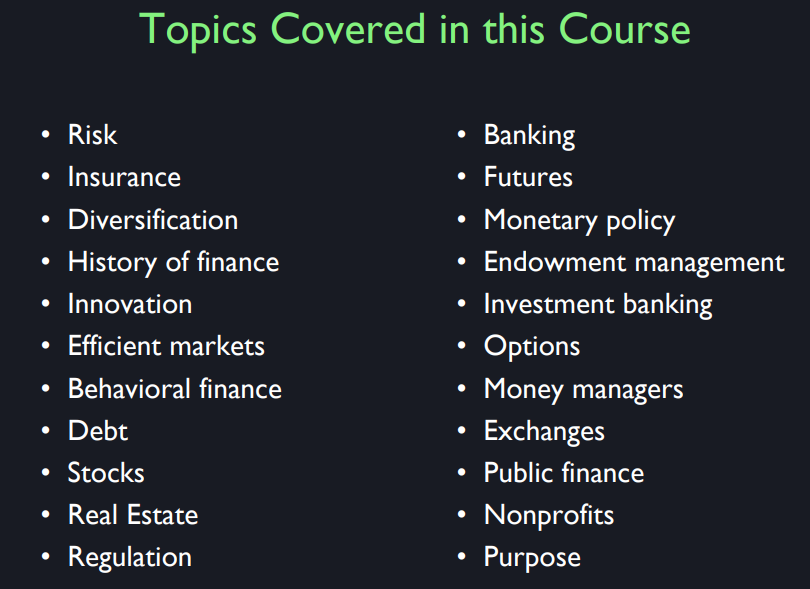
These are the topics in this course. So, risk Insurance, diversification, history of finance, innovation, efficient markets, behavioral finance. Actually, behavioral finance is a little bit more prominent than you might think from its appearance as number seven on this list. Behavioral finance is the application of psychology, sociology, other social sciences to understanding financial events. It’s a revolution in finance that I have watched over the whole course of it because I have organized conferences on behavioral finance starting in 1991, working with Richard Thaler at University of Chicago. We’ve been doing that for 25 years, but we just bequeathed that there are regular seminars of professors too, Nick Barberis here at the Yale School of Management. But we’ll talk about it because I kind of believe in a unity of knowledge.
So this course will differ from many other finance courses in that I want to talk about real people and how things really work. Then we’ll talk about debt, the stock market, the real estate market, regulation. Oh by the way, regulation is an interest of mine too, more so than most people who teach finance because I think that the markets need to be regulated. Human beings have a tendency to be manipulative and tricky, and finance is used to trick people. That’s why we need regulators. So you shouldn’t assume that I want to send you off to Wall Street. I think that you might go to be a member of the right like the Securities and Exchange Commission or something else as a job and be proud of it. OK? It’s important.
And then banking, futures – futures market has a special meaning in finance, monetary policy, endowment management, investment banking, option, money managers, exchanges, public finance, nonprofits, and finally, that last lecture will be on the purpose of all this. So that’s this course. So, I wanted also to just reflect on the relative. I said this course looks more vocational in a way, but I don’t consider this vocational school. This is, I like to say, useful. One thought, perspective I wanted to give you was how important is finance anyway.
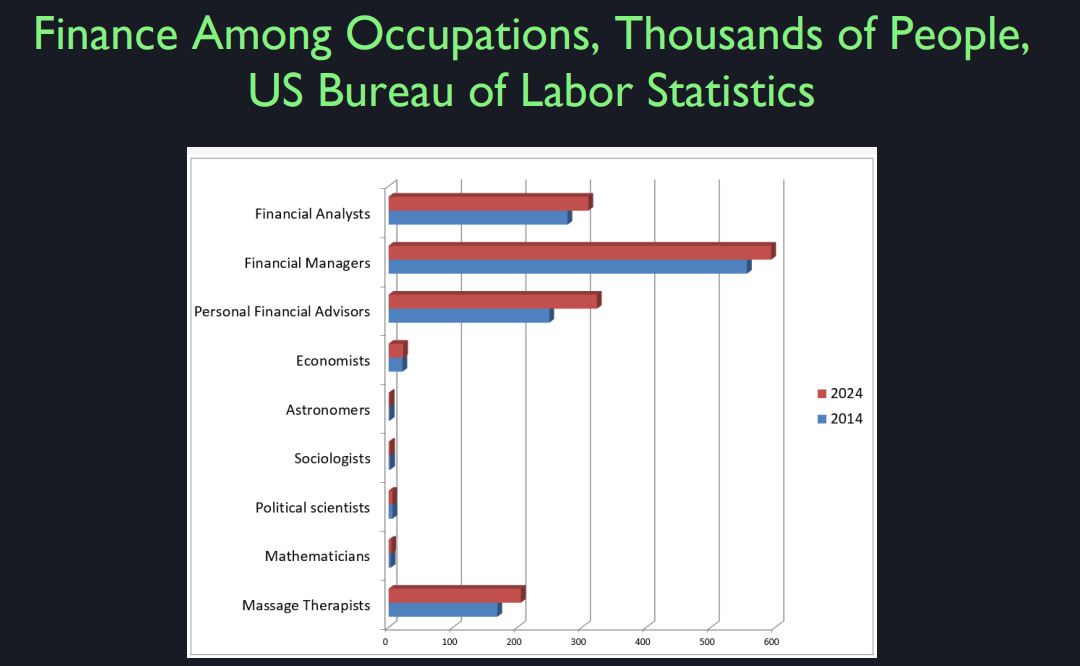
Unless you go into academia, you will get a job somewhere in the real world. So where are the jobs? Well, I looked up on the Bureau of Labor Statistics – it was a publication of the U.S. government. On their website, they have data on just how many people are in different professions in the United States; and they also have a forecast. So what I’m showing – the latest data is for the year 2014, and it has the number of people in thousands. And then also on there we have the projection for 2024. So, you note that at the top I’ve got finance – these are specific finance profession, not all finance professions. Financial analysts, financial managers, personal financial advisors, they all have hundreds of thousands of people. But I wanted you to note, what about the other majors that you have here? I’m not diminishing them. But economics, economists, not so many. But you might also be interested in astronomy – I actually love astronomy. When I was a kid, I thought I’d be an astronomer. But I had to reach reality – there’s lots of exciting fields where there are almost no jobs. How many astronomers are there, sociologists, political scientist, or mathematicians? This is not to diminish your majoring in this field, but you just don’t expect to get a job in those fields. I also put down at the bottom massage therapist, OK? I didn’t know that was a profession, but there is projected to be about 200,000 massage therapists in the United States in 2024. So we don’t have a massage therapy major here, but that’s a sign of how the market makes things important.
Now run up, Farahar might be right about this. There’s something wrong with having so many finance people – maybe we need more massage therapists than finance people. But there’s a sense of reality that I think that part of the reason that there’s so many of them is that they deal with important issues that can’t be quickly, they can’t be more easily solved; we need all these people. That’s why I take some pride in this course in being connected to the real world. There are real job opportunities in finance. And there also I think in the new Industrial Revolution period, they will still be. I think this is one of the fields that is not going to be totally replaced by a computer. The problem with finance is a high inequality in this field. Some people make a lot of money, but on the other hand, you have to give it away. This is another thing about this course. If you make a lot of money in finance, it’s a game, you enjoyed it, now give most of it away – that’s going to be a theme.
Good and Evil
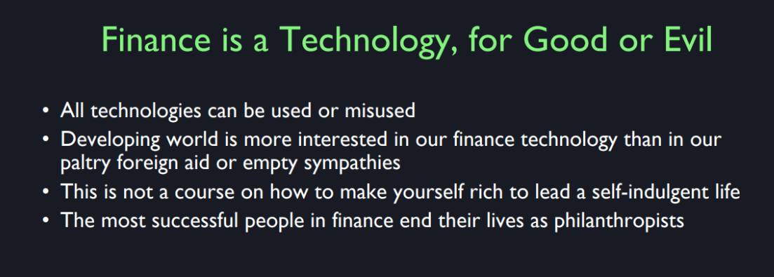
So the idea is, I said this before, finance is a technology,
it can be used for good or evil. It has a tendency for a successful practitioners to
start attracting a lot of money. That doesn’t mean that you can’t be
a moral and ethical person in finance. So one thing I note in giving
talks around the world that when you go to poor countries and
give a talk, they are intrinsically interested in
finance because people today recognize that financial markets
are part of economic success. They understand that in China,
they understand that in Russia, they understand that in Brazil and
many more countries. Because finance is a real technology. They’re not so interested in getting
foreign aid, they don’t need foreign aid, they just need the right principles and
the wealth appear on it’s own.
So this is not a course about how you
can lead a rich and self indulgent life. It’s a course that involves
some moral purpose. Andrew Carnegie was one of
the richest men in America. He said that he thinks that rich people,
people who succeed in business. He doesn’t use the word business. People who succeed in affairs. Now that sounds different today, but
affairs meant business back then. People who succeed are people
with a natural, practical talent. And the business world selects for
people with this natural talent. And so when they make a lot of money it
is their obligation to give it away for the benefit of society and not to their
useless children or spoiled children.
Moreover, Andrew Carnegie said,
you can hear him say this, he said that you should give it away
while you are still young because you’ve amassed all this wealth,
what’s going to happen to it? It’s absurd the story that happens. Young people make a lot of money when
their talents are at their strongest. Then they get old and
they don’t know what to do anymore. They work until they die or
they become self indulgent. And it ends up with their children. And then it ruins the children’s life
because now they have no purpose and they’re just filthy rich. And they just squander it.
So like Vanderbilt and his grandson, William Henry Vanderbilt,
made huge amounts of money. And then his son married a socialite,
the famous Mrs. Vanderbilt, who spent all the money in showing off
her wealth and having big parties. Maybe that was good in some sense,
but you don’t want that to happen. So what Carnegie said is
you have to retire early. And become a philanthropists that’s
the second stage of your life. So I want to come back to this
thing that if you go into finance think of you life as having two states. Like Bill Gates, Bill Gates was
running Microsoft then he retired and set up the Gates foundation and
he’s actively working on giving it away. So this is not a course,
again, repeat, not a course. It’s a course on how you can
make your mark on society, but it’s not a course on how to get rich.
Quiz

Lesson 2
VaR and Stress Tests
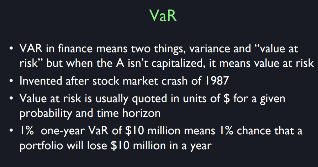
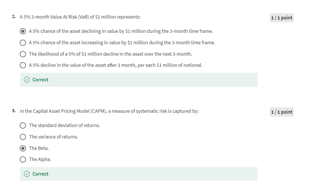
And I just mentioned, there’s something else in finance called VAR. Actually, I have on the slide that it means two things. It means variance and it means value at risk but actually there’s a third one that’s vector autoregression but I don’t… I was just thinking that it can be confusing. So the variance of a portfolio is defined as a measure of it’s variability. In finance, some people use VAR for ‘value at risk’ and this term is relatively new. It didn’t appear until after the stock market crash of 1987. And so, it’s a measure used by some finance people to quantify risk of of an investment or of a portfolio and it’s quoted in units of dollars for a given probability and time horizon.
For example, if it says lets’s say 1%, one-year value at risk of 10 million, it means that there is a 1% chance that the portfolio will lose 10 million in one year. And then, there’s another measure of risk that’s become popular in recent years especially after the financial crisis of 2007-09 and that’s called the stress test.
Now, the term stress test goes back to the 1960s or so and it refers to something that your doctor would order if he was worried about your heart and he would have you get on a treadmill in a medical facility, and run and they have an electrocardiogram hooked up to you and they check out your heart while you’re under stress, the stress of running. But now the term has moved into finance. Office of Federal Housing Enterprise Oversight actually was doing stress tests on Fannie Mae and Freddie Mac before the 2008 crisis. It didn’t work.
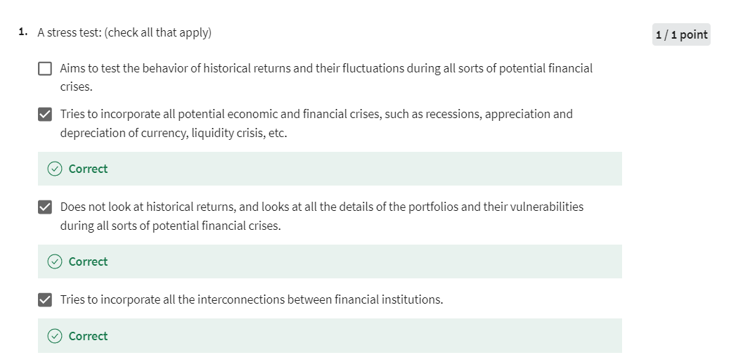
Those two firms both failed but they were trying anyway. So, a stress test reflects the idea. It’s not a basic statistical concept, it’s a measure. It’s a method of assessing risks to firms or portfolios. The idea of a stress test is that, let’s look at a portfolio not just by its historical returns and how variable they are, but let’s look at the details of the portfolio and ask what vulnerabilities there are for various kinds of financial crisis because what actually stresses firms the most are crisis, it’s not just normal variation and this is something I’m going to come back to later in this lecture that there are extreme events occur and so…
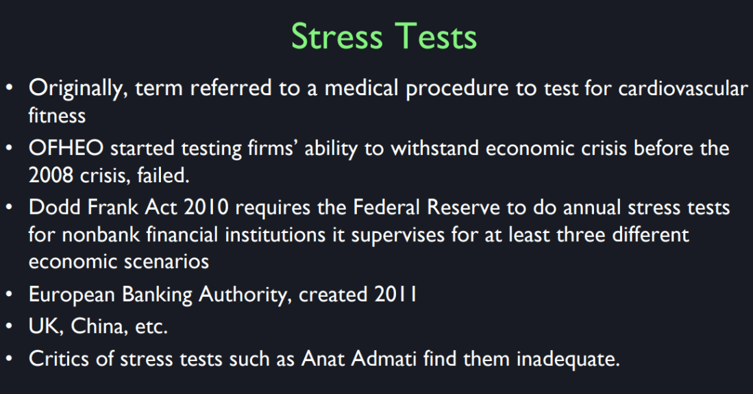
The stress test is a test usually ordered by government to see how some firm will stand up to a financial crisis. The Dodd-Frank Act in the United States of 2010 requires the Federal Reserve to do annual stress tests for non-bank financial institutions it supervises. I think they’re already doing them for banks and they wanted to be at least three different economic scenarios that the Fed would present. What they would do is, they would get information from the firm about all of their interconnectedness with other institutions, everything they own, how safe is it, and they would look at, say for example, what would happen if there were a severe recession, or what would happen if the dollar depreciated or appreciated, or what would happen if there’s a short term liquidity crisis with suddenly ability to borrow money in the short term dries up.
The Dodd-Frank Wall Street Reform and Consumer Protection Act was passed into Federal law on July 21, 2010 as a response to the financial crisis of 2007 to 2008. This Act constitutes the most significant changes to U.S. financial regulation since the regulatory reform that followed the Great Depression. The Dodd-Frank Act didn’t specify what the three different scenarios were, but they did say that there should be at least three. So this is a different story. This is scenario analysis. It’s not something that we’re going to emphasize in this course because it’s…
More institutional details that get into the calculations. The European banking authority which was created in 2011, after the financial crisis, has also instituted regular stress tests for European banks. The United Kingdom, China and other countries all do stress tests now but the question is, do they work? Well, there is a growing amount of skepticism that they can really measure what will happen in the next crisis. Anat Admati is a professor at Stanford who’s been arguing it’s all garbage. You can’t. These guys who are trying to predict what will happen to these companies in a financial crisis, they just don’t have the imagination and understanding of how things work out in a panic, in a financial panic and she thinks that they are just way underestimated.
Generally, the stress test come out saying it’s okay, don’t worry. It does remind me, I was on stage with the chief economist of, Freddie Mac here at Yale. We had a… It was around 2005 and he was boasting about their stress tests. And he said that… So I asked him what if there’s a real estate crisis and home prices fall a lot. They’re company that guarantees mortgages on homes, and so he said, “Well, we have figured out what would happen to our portfolio even under extreme stress situations.” I said, "Well, what is your…? ". I did this on stage not this stage, it wasn’t build yet. I said, “What’s the biggest price decrease you ever considered for your stress test?” They said, “Oh, we considered a 13% drop in home prices.” And then I said to him, “Well, what if it’s bigger than that?” And then he looked chagrined then he said, “We’ve never seen home price drops, not since the Great Depression. You’re not talking about another depression, are you?”. We’re still friends. I still meet him on vacation but the problem is that home prices fell 30% right after that meeting or within a couple of years.
And these two companies, Fannie and Freddie that were considered safe. Well, actually if you read the OFHEO reports on the stress tests back, and they will say, there is some concern still. You know, they’re hedging, but basically they said don’t worry and so that was the end of OFHEO. The government shut it down. So the question is whether we can do it this time. So Anat Admati doubts that we can do this time. She thinks there are bigger worries. The stress tests are all coming out as no problem but now she’s not so sure. If I were the CEO of a firm, I imagine I would ask for stress tests and doing it internally, but you don’t want it public. What if it comes out bad? See, the problem is if you ever release that information then all of your other companies that might do business with you are worried about that and so they wouldn’t want to do business with you. So, it’s like your reputation is at stake. So if the government demands that you reveal information for a stress test, you have every incentive that you try to whitewash it. And so the question is whether the regulators have enough incentive to demand and push. The Dodd-Frank Act gave regulators, the Office of Financial Research subpoena power, so they can go in there and demand information from firms. But it’s hard to get it I think. In the real world it’s a battle. They don’t want to tell you.
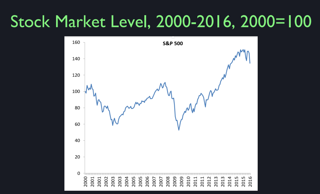
S&P 500
This is the S&P, Standard & Poor’s 500 stock price index and it’s used as a benchmark for returns. So this is what you did if you just invested in the whole market monthly from 2000 to 2016. And what it shows is quite a roller coaster ride of value, right? So, actually, I should have maybe plotted it longer. It was rising for a long time before that and then it had a huge drop from 100 it fell about in half. And then starting in 2003 it started a long increase again. And then here is the great financial crisis, 2007 to 2009. And then since then, has been going up a lot here. You know, from here to here, this is 2009. From here to here it tripled in value. It’s amazingly unstable, the stock market. To think that the risk of any other comp, the Law of Large Numbers is not working here because this is the Standard & Poor’s 500 Index. It’s an average of 500 stocks. So if they were all independent of each other, the Law of Large Numbers would make the stock market as a whole almost constant. But, in fact, it’s actually gone up hugely. So there’s definite dependence across stocks. But I’m not going to be focusing on forecasting the stock market here. We’re going to make the assumption that it’s very hard to forecast. So we’re going to look at risk as something that we can quantify by looking at the standard deviation of past risks and not focus on what’s new right now.
Now what I want to do next is to look at one firm within the S&P 500. What do you think it looks like if I were to plot Apple on the same chart here? Did you ever heard anything about how they performed? With that? Does anyone know how Apple has performed since 2000? I guess we’re not an eager class of stock market devotees. Yes you did, yeah. Pretty well since the release of the iPhone, that’s around 2007. You said pretty well, since the release of the iPhone. And, was it 2007? They did a series of releases of new different models. You’re right. They did pretty well. So I’ll show you what pretty well mean. I’m going to superimpose on the same plot, Apple OK. That’s Apple.
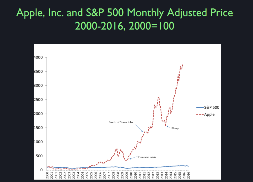
It looks different because I had to scale down to fit Apple onto it. So this is quite a good performance because I started both, re-scaled both of them, they started at 100 and it’s now, what is that? 3,500, 3,600, something like that. So that means a 30, say a 40 fold increase in value in 15 years. So imagine that you were taking this class in 2000. I was teaching this class, maybe 15 years ago. But imagine that you were taking this class then. And, you came home to your parents and said, “You know, I think Apple’s stock is a great investment. I just have a quick request of you. Could you take out a second mortgage on the House, borrow $400,000 and put it into Apple’s stock?” Well, if you did that in 2000, your parents would now own over $15 million. The problem is, what’s the problem with that? The problem is nobody knows the future. If you knew that Apple was going to do that, you would have obviously done that. But nobody knew that Apple was going to do that. So you had also faced some problems with your parents if you did that, because starting in 2000, Apple dropped quite a bit and you lost it’s like three quarters of your money. It’s hard to tell here right. It was really limping along for four years.
So you come back four years later and your parents say, “Do you realize what you did? You’ve made us borrow $400,000. And now it’s just, we’re down to $100,000.” But then you have to be convincing again. No. Just hang in there. This is the problem with investing. Hang in there please. And then it start recovering slowly. Yeah I think back then, this is before the iPhone. Here back in 2000. One, two, and three. It looks like Apple was washed up. When did they bring Steve Jobs back? Anyone know that? Anyone read about? I’m assuming you know who Steve Jobs is. Steve Jobs was the founder of Apple Corporation. And he was kind of a difficult guy and kind of quirky. So they fired him. It was his own company, but you can get fired from your own company. And they put in some professional management, whereas he was kind of a little bit strange. The professional management did this. They brought it down to a low value. And then they invited Steve Jobs back. They thought maybe he does have some kind of genius. But they’re still doing well after his death.
So maybe it’s, you know, the company develops a sort of culture and a spirit that allows them to keep doing. I really think that’s true about organizations. They go on for so long. Sometimes it’s a great success. So for example, the Economist magazine was founded in London in the early 19th century and it was, it’s still a great magazine. How can they last so long? I went and visited them once and I discovered that they don’t even put by lines. They have a different culture. They usually don’t put by lines on articles. In other words, if you were to work for the Economist as a writer, you will not become known. They will not put your name, print your name on the articles you write. So how can they do that? Because young people want to establish themselves somehow. But they do. And It’s a different culture at the Economist magazine as a result. So every company has its own culture and it produces a strange outlier effect.
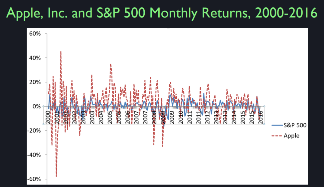
This is the return on Apple’s stock, in red, the red dash line and the return on the S&P, Standard & Poor’s 500 stock price index. So you can see that the returns on Apple have been very variable. Much more variable than the return on the S&P 500. In fact, when you look at this it’s hard to judge from this picture which one did better, right? It looks like Apple is going up and down all the time. It’s this noisy, really noisy. And the aggregate stock market looks tanned by comparison. It’s hard for you to judge which one did better. But you see maybe, if you look you can sort of tell that there are more ups and downs. But it’s so noisy from month to month. These are monthly returns. So here last time Apple lost almost 60 percent in one month. So it was horrible.
The other thing is I don’t know if you can tell that it’s correlated with the S&P 500. That when the S&P 500 moves up, it moves up and when the S&P 500 is down, for example. But, see, this is the experience of investing is puzzling because the noise dominates. It is so scary watching these things go up and, if you take an interesting investment like Apple, it just goes up and down so much from month to month. And, it could be under for years and you can really lose faith in your acumen after it’s going badly for years.

So, this is just the variance of Apple versus the variance of S&P 500. The standard deviation of Apple capital gain was 12.8 cents a month. That’s not annualized. Annualizing means multiplying it by 12. This is a scatter diagram showing the returns on the S&P 500 on the horizontal axis and the returns on Apple on the vertical axis. And you can see that the scatter has an upward slope to it which means they’re correlated. It’s not that strong an upward slope, but when S&P is high, Apple tends to be high in return and when the S&P is low, Apple tends to be low. But it’s more variable. But this goes from +60 to -80. And on this axis I have -50 to +50. So Apple is more variable than S&P 500. But you can see that there is a correlation.
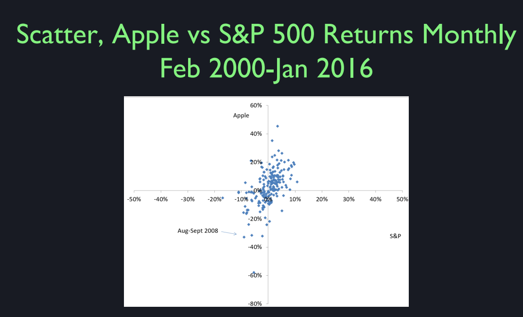
Actually it’s better if I put a regression line in. This is a line fitted through the scatter points. And it shows it has a slope of 1.45 which is greater than one, which means that Apple overreacts to what happens in the aggregate stock market. And then it has noise on top of that. Apple noise, like Steve Jobs death noise that doesn’t affect the overall stock market.
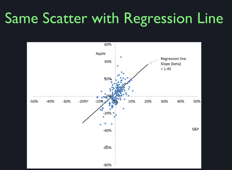
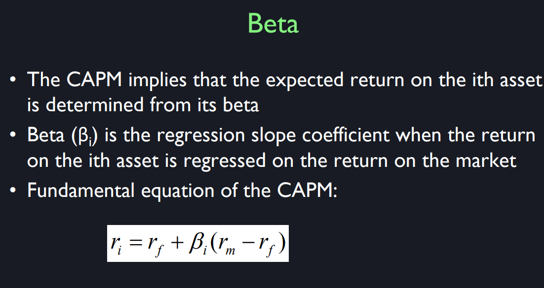
So Apple actually, this is going to be a fundamental concept and as far as the beta of a stock is a measure of how it relates to the stock market. If the beta is one, then the asset tends to go up and down one for one in terms of returns with the aggregate market. If the beta is two, well, they’re kind of rare to see beta two stocks. Beta 1.45 is getting high. So the Apple reacts more than directly to the stock market. So when times are good, people think they are really good for Apple. And when times are bad they think it’s really bad for Apple.
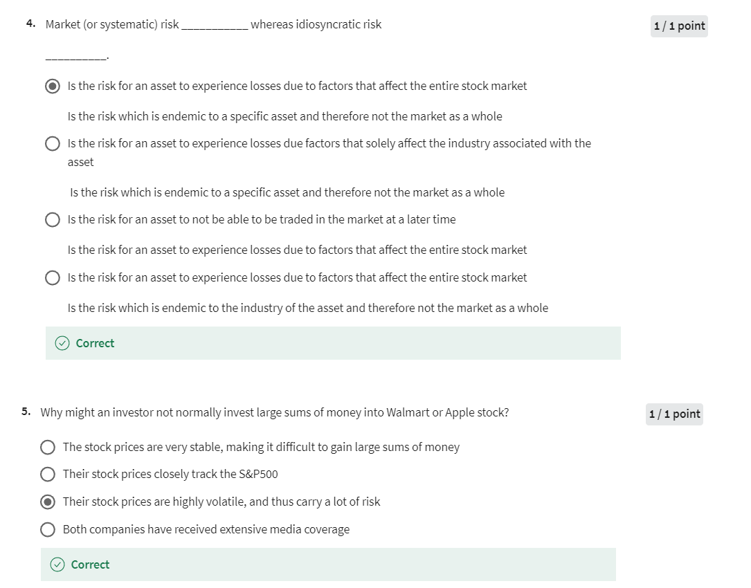
The concept here is market risk versus idiosyncratic risk. So market risk is the risk of the whole stock market. And for an Apple investment, the market risk of that investment is the risk that Apple will do something in reaction to the aggregate stock market. But idiosyncratic risk is Apple only risk. So that would be the death of Steve Jobs, or the iFlop the iPhone that nobody liked. That occurred. So they make mistakes and they take risk. The people at Apple have a history of taking risks. They’ll try something that might not work out. They don’t always work out, but on an average, they do.
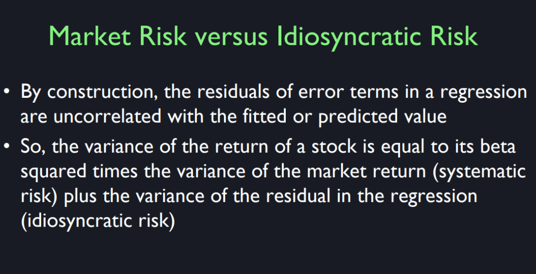
So the variance of the return on a stock is equal to it’s beta squared times the variance of the market return and that’s called systematic risk. Plus the variance of the residual and the regression, the residual in this regression.
I think some of this might be, new, our graduate students can clarify some of these concepts for you. A regression line is a single line that best fits the data in your scatter plot. So how is this calculated? Imagine you have a scatter plot with 50 dots and you start by drawing a line through them. The vertical distance between a given dot and the regression line is that dot’s residual. Also known as the error of your proposed line with regard to that single dot. So, to get a better fit I can try changing the slope or a constant parameter to force the line to go perfectly through dots one and two, but that will make the residual associated with dot three really big. So what do we do? We want to minimize some combination of all 50 residuals. So statistics proposes the least squares method. What do the different slopes mean? Remember the equation for a line in algebra class. y = mx+ B. The slope m is how much y changes for a 1 unit increase in x. In finance we call y as the return on Apple stock, x as the return on the market, slope m as beta, and the constant B is Alpha. Slope beta tells how much a particular stock co-moves with the market and thus as a measure of the stock systematic risk.
So the idiosyncratic risk is the risk that the point will lie above or below that line. And you can see, there’s a lot of idiosyncratic risk for Apple.
Joe McNay Story
All right,
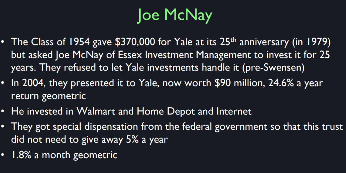
I want to tell you another story. This is a Yale story. Joe McNay, I think he was a Yale graduate. The class of 1954 was celebrating
the 25th anniversary of their graduation, that would be in 1979. And somebody said, this guy,
Joe McNay is a great investor. Why don’t we, as a class,
give money to Joe McNay, and just ask him to invest it for 25 years, and turn
it over to Yale University as our gift. But we don’t turn it over now,
because apparently they thought that the Yale portfolio was
not managed well at all. And so this is before David Swenson
became the head of the Yale portfolio. So Yale was investing in government
bonds and safe things like that. They couldn’t stomach the variation
that you see in investments. But Joe McNay was just this creative guy. And they said hey, you know, this is just
our celebration for our 25th anniversary. We don’t care about this 370,000. We want you to invest it for
maximum returns, and you can take chances. We’re in the mood. Hey we’re all having our beers
together 25 years later. It’s It isn’t often that investors will
tell that to an investment manager. So, right? You don’t say,
if you lose all of it, well, okay. We don’t care. But we think you can do it so please try. So, Joe McNay invested it in Walmart
Home Depot and some Internet stocks. [LAUGH] So, he took Walmart, it’s like
an Apple corporation, really volatile. He thought,
well they’ve told me I could do this. And so he gave to Yale University
$90 million, quite a success.
Distribution and Outliers
Now the question is, I was already suggesting that there is an issue of outliers. So, what do we mean by an outlier? Well, there’s something, I’m sure you’ve heard about the normal distribution or the bell shaped curve for random variables. The normal distribution is a typical distribution for random variables in nature and there are reasons to think that many random variables follow a distribution like this. The distribution has two parameters, its mean and its standard deviation. So in this case, I have plotted it for two different standard deviations but both a mean of zero. So, this is a theoretical probability distribution for let’s say a return on a stock and here the standard deviation is one on this pink curve, and it’s three on the blue curve. Many random variables in nature follow this distribution but not all of them and that’s important because in finance it tends not to follow this distribution, that we tend to have outliers or fat tails.
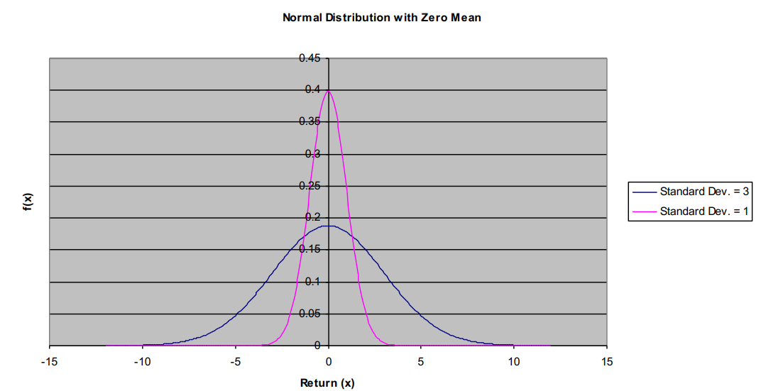
The normal distribution, has two tails. This is the right tail which has high values of the random variable, and here’s the left tail which is low values of the random variable. And the height reflects the probability of getting that value. So, if this were the distribution of returns for Apple stock, and let’s say, a standard deviation of three percent, then the probability of getting a return of three percent is pretty good. Here’s three percent, and the probability of getting three standard deviations, that would be nine. You can see it’s just about negligible, and then I don’t even show it anymore. The probability of four standard deviations out is essentially zero. That’s what the normal distribution says. The normal distribution has been used to describe for example, human heights or human IQs or SAT scores or, lots of things seem to follow the random normal distribution. And you probably have become intuitive about this. If you see some random variable repeatedly, and it’s pretty much always been between say minus five and plus five, then intuitively you start to think it can’t happen, that it would be 15 because you’re intuitively trained by life’s experiences.
柯西分布(Cauchy distribution)是一种连续概率分布,以法国数学家奥古斯丁·路易·柯西(Augustin-Louis Cauchy)的名字命名。柯西分布在统计学和概率论中有一些独特的性质,使它在某些应用中非常重要。
柯西分布的概率密度函数(PDF)定义如下:
[ f ( x ; x 0 , γ ) = 1 π γ [ 1 + ( x − x 0 γ ) 2 ] f(x; x_0, \gamma) = \frac{1}{\pi \gamma \left[1 + \left(\frac{x - x_0}{\gamma}\right)^2\right]} f(x;x0,γ)=πγ[1+(γx−x0)2]1 ]
其中,( x 0 x_0 x0) 是位置参数,确定分布的中心;( γ \gamma γ ) 是尺度参数,确定分布的宽度。
柯西分布有以下几个显著特性:
没有期望值和方差:柯西分布的期望值和方差都不存在。这与大多数常见的概率分布不同。例如,正态分布有明确的期望值和方差。
厚尾:柯西分布的尾部比正态分布更厚,这意味着它在尾部有更高的概率质量。也就是说,它在极端值(远离中心)出现的概率较高。
标准柯西分布:当位置参数 ( x 0 = 0 x_0 = 0 x0=0 ) 且尺度参数 ( γ = 1 \gamma = 1 γ=1 ) 时,柯西分布被称为标准柯西分布,其概率密度函数简化为:
[ f ( x ; 0 , 1 ) = 1 π ( 1 + x 2 ) f(x; 0, 1) = \frac{1}{\pi \left(1 + x^2\right)} f(x;0,1)=π(1+x2)1 ]
特例:柯西分布是一个特例的斯图登特t分布,其中自由度为1。
对称性:柯西分布是对称分布,分布曲线在 ( x 0 x_0 x0 ) 处对称。
柯西分布在物理学中有一些应用,例如描述共振现象。此外,由于其厚尾特性,柯西分布也在某些金融模型中用于捕捉极端市场行为。然而,由于其期望值和方差不存在,它在统计推断中相对不常用。
The Cauchy distribution is a continuous probability distribution named after the French mathematician Augustin-Louis Cauchy. It has some unique properties that make it significant in certain applications within statistics and probability theory.
The probability density function (PDF) of the Cauchy distribution is given by:
[ f ( x ; x 0 , γ ) = 1 π γ [ 1 + ( x − x 0 γ ) 2 ] f(x; x_0, \gamma) = \frac{1}{\pi \gamma \left[1 + \left(\frac{x - x_0}{\gamma}\right)^2\right]} f(x;x0,γ)=πγ[1+(γx−x0)2]1]
where ( x 0 x_0 x0 ) is the location parameter, which determines the peak of the distribution, and ( γ \gamma γ ) is the scale parameter, which specifies the half-width at half-maximum.
Key characteristics of the Cauchy distribution include:
No Mean and Variance: The Cauchy distribution does not have a defined mean or variance. This is in contrast to many common probability distributions, such as the normal distribution, which have both a well-defined mean and variance.
Heavy Tails: The Cauchy distribution has heavier tails compared to the normal distribution, meaning it has higher probabilities for extreme values. This implies that it is more likely to produce outliers.
Standard Cauchy Distribution: When the location parameter ( x 0 = 0 x_0 = 0 x0=0 ) and the scale parameter ( γ = 1 \gamma = 1 γ=1 ), the distribution is known as the standard Cauchy distribution. Its PDF simplifies to:
[ f ( x ; 0 , 1 ) = 1 π ( 1 + x 2 ) f(x; 0, 1) = \frac{1}{\pi (1 + x^2)} f(x;0,1)=π(1+x2)1]
Special Case: The Cauchy distribution is a special case of the Student’s t-distribution with one degree of freedom.
Symmetry: The Cauchy distribution is symmetric around the location parameter ( x 0 x_0 x0 ).
In terms of applications, the Cauchy distribution is used in physics to describe resonance phenomena. Its heavy-tailed nature also makes it useful in some financial models to capture extreme market behaviors. However, due to the lack of a defined mean and variance, it is less commonly used in statistical inference.
But in fact, there are other distributions that are more characteristic of financial returns. So there’s another kind of distribution called the Cauchy distribution after a famous mathematician. And what I’m showing here is, at 100 draws from the normal distribution in blue, and 100 draws from the Cauchy distribution in red. Now you see the difference between a Cauchy and the normal. The normal distribution has a kind of look to it, you see it’s going up and down about the same amount all the time, well, I’m not saying that’s exactly right. The probability that it will be 10 times the normal change, the usual change is negligible so you never see it deviating from… It has the kind of uniform look to it through time but with Cauchy, it also looks very much like normal. You can’t even tell them apart for long intervals of time and then bang! there’s some big positive value. In other words, the distribution under Cauchy is fat tailed so the Cauchy looks like a normal distribution except instead of just trailing off to zero, the distribution continues out above zero, way out.
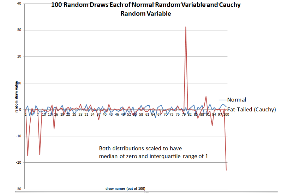
So, you can be deceived by a fat tailed distribution like the Cauchy into thinking that you’re living in a fairly stable world whose risk I understand, but the problem is, there are these big events that occur from time to time.
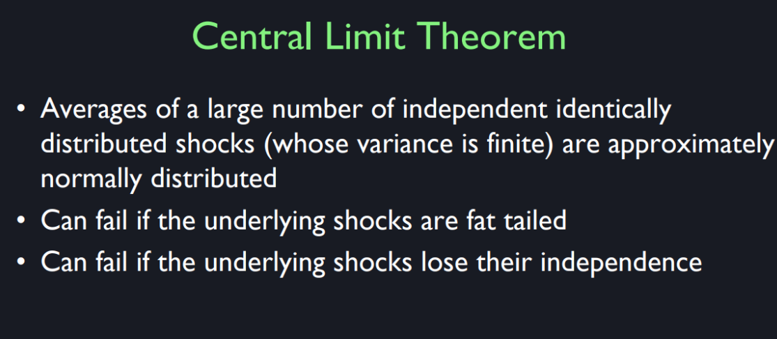
The Central Limit Theorem in Statistics says that, averages of a large number of independent identically distributed shocks or random variables is approximately normally distributed, but that central limit theorem assumes that the underlying shocks do not have fat tails. So, if you’re taking the average of stock market returns which tend to be fat tailed, then your average is not a good indication of the real average over long intervals of time because you might well have gotten a sample where none of the fat tail outlier stocks.
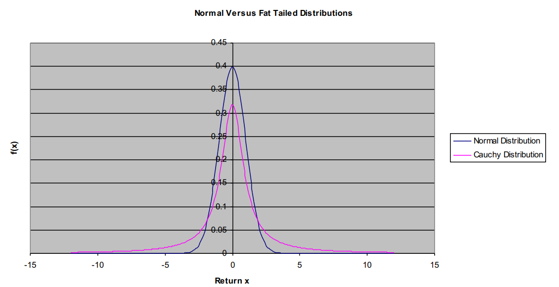
My friend Nassim Taleb has written a book called “The Black Swan” which got a lot of attention. It referred to black swan events. So you’ve seen a lot of swans in your lifetime, and they’ve always been white, right? Have you ever seen a black swan? You might well conclude that black swans do not exist but in fact they do exist. There are black swans and so that’s a metaphor he uses for a fat tail. Here is a plot of the normal and the Cauchy distribution. The Cauchy distribution looks pretty much like the normal. It’s a bell-shaped curve and it trails off but there’s a subtle difference, that there are these rare very… they’re not quite as rare as as the normal would suggest. The real world puts fat tails in our lives.
Here is a plot of the histogram of daily stock price changes since 1928. And what I have, what this thing is, how many days are there since 1928, but it’s tens of thousands of days. And so what we’re seeing here is that the stock market yielded a return of, this is for the S&P 500, or extended S&P 500 of between, I guess this is between… of one percent with some interval around that. It did that and suddenly like 9,500 days, it earned plus one percent one day. And then, on something like 2,500 days, it earned plus two percent. And then on Sunday like 800 days, it earned plus three percent and looks like it’s about, I don’t know, 400 days it was plus 4 percent. And then here, I can’t even figure that out, something at plus five. After that, they looked like you can’t even see them anymore.
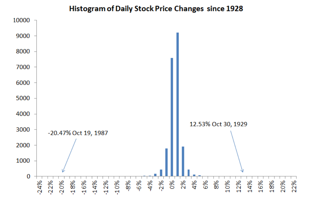
So you might conclude by looking at this histogram that stock market returns are always between say minus six percent and plus six percent. A matter of fact, on October 30, 1929 the stock market went up 12.53 percent in one day. And on October 19, 1987 the stock market fell 20.47 percent in one day. It was quite a shock. By the way, on this day I was lecturing giving my…this class I was teaching ECON 252, and one of the students was listening to a transistor radio. Do you know what a transistor radio is? It’s what they used to have before you had iPhones and things like that. So he raises his hand, I will never forget this, and he said, “Did you know the stock market is crashing right while you’re giving this lecture?”.
So, instead of going back to my office, I just thought, “What is he saying?” I went downtown and I talked to my stockbroker, Merrill Lynch, right here in New Highland. I took the elevator up and just walked in on there just to see what was happening. And it was this turmoil and everyone, I did manage because I walked in. If you tried to call your broker, you couldn’t. He wouldn’t answer, he’s too many calls but I walked in, barged in on him and I said, “What’s happening?” And he said, “Don’t worry, don’t panic. There was this big event, horrible event.”. That was the biggest drop, one day drop, ever in the whole history of the U.S. stock market so I had the good fortune to be warned of it by my student with the transistor radio. The fact that my student, this is before laptops, but he did…we had problems with transistor radios back then.
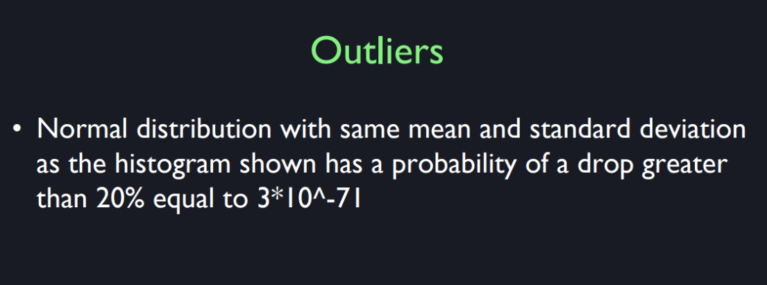
So that’s an outlier. The normal distribution with the same mean and standard deviation as this histogram says that the probability of a drop greater than 20 percent is equal to 3*10^-71. That’s awfully close to zero if you know. I think that the estimated number of atoms in the universe is bigger, that’s 10^80 but it’s getting on like that. So, it’s essentially zero but it’s wrong because it happened and I was there. I saw it happen and I saw the excitement that it generated.
Chalk Talk - Covariance
The idea of covariance. When you have two separate stocks,
for example. >> Okay. [COUGH] I’ll try to start
keeping things really simple. There’s two different companies. They’re both startups and they’re
both trying some risky new venture. And they both,
it’s like a coin toss, right? They both have a 50,
50 chance of succeeding. And if they succeed they’re
worth a million dollars, and if they fail they’re worth zero dollars. So we have two probability distributions, one for the stock one, right? This is one million and
this is zero and this is 0.5. I’ll leave it at 50, 50 for now. And this is stock two, 0, 1, 0.5. So it looks the same. [COUGH] Now the question is, are these
two businesses really independent?
We’ve shown their
probability of succeeding. But if I’m going to invest
in both of them as a smart venture capital firm might do,
what do I make of that? Are they the same or different? So let’s say the mean is 0.5 for
both of them. It’s like a fair coin toss, all right? And so, they will deviate
either plus 0.5 for the mean, or minus 0.5 for the mean, both of them. Now but the question I want to
know as an investor, are they going to do the same, or
are they independent of each other? There’s four possibilities,
the covariance, C-O-V, covariance between the two returns is probability rate average of,
so now it gets to variance. But it’s between two companies. So let’s consider,
what’s the first possibility? They both succeed. So it has a 0.25, one and four chance of being a half
above the mean for both of them. So that’s 0.5 times 0.5, right? And then it has a 25%
chance of both being 0. So it’s 0.25 times -0.5 times -0.5. But then there’s the chance that one of
them succeeds and the other one doesn’t. That has a probability of 0.5, because
there’s two different ways it can go. >> Right.
It could be A, that succeeds and B, fails or otherwise. So we have 0.5 probability of -0.5 times 0.5. So what does that add up to? It adds up to 0 right? Because these are both positive numbers,
but these are 1. So the product -0.5 times -0.5 is plus. And so, this is equal to
a half times a quarter, right? The two terms here. >> Right.
And that’s the same here, but with a minus sign, so it cancels out. So if they’re really independent
like that then the covariance is 0. >> Okay.
And we like that as investors,
we don’t want to get in trouble. So we want to see
an independent investment. But on the other hand it could be that
the two companies are really the same, they really betting on the same idea. And so, these are not possible, all right? This probability goes from 0.5 to 0. And then this probability goes to 0.5, and this probability goes to 0.5. >> I see. >> So now we have a covariance of 0.25. It’s not 0 anymore, and that’s a flag that there’s danger here. And the other possibility is that
they’re exact opposite of each other. Only one of the two will succeed,
one will succeed and the other fails. And that would be a negative covariance.
So these things matter, and they become central to our theory
in the capital asset pricing model. This is something that is not in the habit
of thinking of most amateur investors. They look at their investments
one at a time, and they don’t, you always have to go back and
say, what’s the covariance? That’s what really matters for
what happen to your portfolio. Because when you invest in a lot of
companies that are all the same, you’re asking for trouble, because the
whole thing is going to either blow up or succeed. And you can’t live like that. You have to be looking for low covariance. The theory of capital S
pricing theory tells you how to take a count of covariance. >> Okay, so then really this
covariance kind of changes based on how we assign the probability
of each pair of outcomes occurring. So what’s the probability
of them both succeeding? Here we put 0.5. And what’s the probability of them both,
which is like 0 and 0, so that would be 0.5. And we gave no probability to the case
where one succeeds and one fails. So that kind of, is the fact that
the covariance is positive is kind of indicating that these
two stocks tend to do this. They move in the same direction. >> Right.
But they’re kind of simultaneously moving in the same direction. >> So this is the basic bottom lesson. Risk is determined by covariance. >> Right.
Especially if you hold a large number of assets. Idiosyncratic risk just doesn’t matter. It all averages out. It’s this kind of thing where they do the
same thing that you have to worry about. And this is a basic lesson in finance. It just doesn’t come naturally to
most people, you have to ponder this. >> So that’s really interesting, because
when we come to finance most people think of that risk is just
the variance possibly. But actually we’re saying it’s
actually more granular than that. It’s actually the covariance of a stock
with, let’s say the broader market. >> Well yeah, because any investor has
the option of investing in everything. >> Right.
Because there are mutual funds hat will do, there are world funds that put
their money all over the world And so, why shouldn’t you do that? It sounds like it’s a pretty
good thing to do actually. But the one thing they can’t get rid of
is the market risk for the whole world. That’s there,
because if you hold the whole world, you’re still subject to the world’s risk. But that’s what an investor
needs to be focused on, and this is a bad habit among
many individual investors. They just look at one stock and
they think, I’m going to put all my money in that. >> Right. >> And they just don’t consider
how many different options for risk spreading they have in this
vast world that we have around us. >> Okay, and this idea seems very
quite similar to when we were talking before about the market
return versus Apple and we had-
It is.
So then we had different betas, and
so that’s kind of getting at covariance- >> In fact the beta of the i stock is its covariance-
Okay. >> With the market. Divided by the variance of
the return on the market. It’s just a scaled covariance. >> Okay? >> And the average beta has to be one, because I could substitute
the average return on the assets. And that’s the return of the market, so then the covariance of anything with
itself is equal to the variance. It just equals one. >> Okay.
So then, if you’re more than that versus less than,
I see, okay.
So you want to be careful. In other words, the basic says, that the market demands higher
returns from higher beta stock. That means high covariance
with the market stock. And they’re willing to take no
returns if the beta is low, because that means it’s less
contributing to risk in the portfolio. >> Okay. >> In fact, if you can find a negative
betta stock, or lets say goals, it may not always be negative data. But lets say in theory
it is negative beta. Putting gold into your portfolio,
it has no return at all. It doesn’t pay dividends, nothing. >> Right.
But it moves opposite your other investments. That’s the theory. >> Okay, and
everything we’re talking about here, we have this presumption
that we’re all risk averse. And so, I just want to state that’s a key part to why we
care about covariance. >> Yeah. >> But
if there’s somebody like George Soros or Warren Buffett,
maybe they’re less risk averse. >> I have no fundamental insights into
either George Soros or Warren Buffett. My guess is though,
that they have this theory firmly in mind, and they may want to take risks at times. See, the real world is not so
cut and dried as I showed here, but we know the probability of everything. So they may disagree with other people,
and maybe they’re smarter,
maybe they work harder. >> Right. >> So
they won’t always minimize their risk. The CAPM model is an abstraction,
an idealization. And it assumes that there are well-defined
probabilities for everything. But in fact, I don’t think anyone behaves
entirely in accordance with this model. I’m thinking of it as, it’s actually a fabulous model as a first
step in thinking about financial markets. Because it can prevent you
from making a lot of mistakes.
Key Points of the Discussion
Covariance Concept:
- Covariance measures the degree to which two random variables change together.
- In the context of stocks, it indicates how the returns of two stocks move in relation to each other.
Independent vs. Dependent Stocks:
- Two stocks are considered independent if the outcome of one does not affect the other.
- Covariance of zero indicates independence.
- Positive covariance means the stocks tend to move in the same direction.
- Negative covariance means the stocks tend to move in opposite directions.
Example Scenario:
- Two startups with 50/50 chances of success or failure.
- If their successes/failures are independent, the covariance is zero.
- If their successes/failures are dependent, the covariance is positive.
Investment Implications:
- Investors prefer low or zero covariance between investments to spread risk.
- High covariance increases risk as investments tend to move together, leading to higher overall portfolio volatility.
Capital Asset Pricing Model (CAPM):
- CAPM uses the concept of covariance to determine the expected return of an asset.
- Beta is a measure derived from covariance, representing the asset’s sensitivity to market movements.
- Higher beta means higher risk and higher expected return.
- Lower beta indicates lower risk and lower expected return.
Risk Management:
- Individual stock risk (idiosyncratic risk) averages out in a large portfolio.
- Systematic risk, influenced by market-wide movements, is what remains and needs to be managed.
- Diversification is key to managing risk by reducing covariance among investments.
Practical Considerations:
- Investors should focus on covariance and beta to understand and manage portfolio risk.
- Theoretical models like CAPM provide a framework but real-world decisions may require additional insights and considerations.
Key Knowledge Points to Note
Covariance Calculation:
- Covariance between two stocks can be positive, negative, or zero.
- It is calculated as the average of the product of their deviations from their means.
Beta:
- Beta is the ratio of the covariance of a stock with the market to the variance of the market.
- It is a measure of how much the stock’s price moves with the overall market.
Diversification:
- Spreading investments across assets with low or negative covariance reduces overall risk.
- Mutual funds and world funds are examples of diversified investments.
Systematic vs. Idiosyncratic Risk:
- Systematic risk affects the entire market and cannot be diversified away.
- Idiosyncratic risk is specific to individual assets and can be minimized through diversification.
Practical Advice
- Always consider the covariance of potential investments within your portfolio.
- Aim for a diversified portfolio to minimize risk.
- Understand and utilize concepts like beta and CAPM for better investment decisions.
- Remember that theoretical models are guides; practical decisions may require deeper analysis and intuition.
This discussion emphasizes the importance of understanding covariance and risk management in portfolio theory, particularly in relation to the CAPM and diversification strategies.
Covariance Calculation Formula
The covariance between two random variables (X) and (Y) is given by the formula:
[ Cov ( X , Y ) = 1 n ∑ i = 1 n ( X i − X ˉ ) ( Y i − Y ˉ ) \text{Cov}(X, Y) = \frac{1}{n} \sum_{i=1}^n (X_i - \bar{X})(Y_i - \bar{Y}) Cov(X,Y)=n1∑i=1n(Xi−Xˉ)(Yi−Yˉ) ]
Where:
- ( X i X_i Xi) and ( Y i Y_i Yi) are the individual samples of (X) and (Y).
- ( X ˉ \bar{X} Xˉ) and ( Y ˉ \bar{Y} Yˉ) are the means of (X) and (Y), respectively.
- (n) is the number of data points.
Alternatively, for population data:
[ Cov ( X , Y ) = ∑ i = 1 n ( X i − X ˉ ) ( Y i − Y ˉ ) n \text{Cov}(X, Y) = \frac{\sum_{i=1}^n (X_i - \bar{X})(Y_i - \bar{Y})}{n} Cov(X,Y)=n∑i=1n(Xi−Xˉ)(Yi−Yˉ) ]
For sample data, the formula is slightly adjusted to use (n-1) instead of (n):
[ Cov ( X , Y ) = ∑ i = 1 n ( X i − X ˉ ) ( Y i − Y ˉ ) n − 1 \text{Cov}(X, Y) = \frac{\sum_{i=1}^n (X_i - \bar{X})(Y_i - \bar{Y})}{n - 1} Cov(X,Y)=n−1∑i=1n(Xi−Xˉ)(Yi−Yˉ) ]
Beta Calculation Formula
Beta (( β \beta β)) of a stock (or an asset) is a measure of its sensitivity to the overall market. It is calculated using the covariance of the stock’s returns with the market returns divided by the variance of the market returns:
[ β = Cov ( R i , R m ) Var ( R m ) \beta = \frac{\text{Cov}(R_i, R_m)}{\text{Var}(R_m)} β=Var(Rm)Cov(Ri,Rm) ]
Where:
- ( R i R_i Ri) represents the returns of the individual stock.
- ( R m R_m Rm) represents the returns of the market.
- ( Cov ( R i , R m ) \text{Cov}(R_i, R_m) Cov(Ri,Rm)) is the covariance between the returns of the stock and the market.
- ( Var ( R m ) \text{Var}(R_m) Var(Rm)) is the variance of the market returns.
Expanded Formulas
Covariance Expanded:
[ Cov ( X , Y ) = 1 n ∑ i = 1 n ( X i − X ˉ ) ( Y i − Y ˉ ) \text{Cov}(X, Y) = \frac{1}{n} \sum_{i=1}^n (X_i - \bar{X})(Y_i - \bar{Y}) Cov(X,Y)=n1∑i=1n(Xi−Xˉ)(Yi−Yˉ) ]
Where:
- ( X ˉ = 1 n ∑ i = 1 n X i \bar{X} = \frac{1}{n} \sum_{i=1}^n X_i Xˉ=n1∑i=1nXi)
- ( Y ˉ = 1 n ∑ i = 1 n Y i \bar{Y} = \frac{1}{n} \sum_{i=1}^n Y_i Yˉ=n1∑i=1nYi)
Beta Expanded:
[ β = ∑ i = 1 n ( R i − R i ˉ ) ( R m − R m ˉ ) ∑ i = 1 n ( R m − R m ˉ ) 2 \beta = \frac{\sum_{i=1}^n (R_i - \bar{R_i})(R_m - \bar{R_m})}{\sum_{i=1}^n (R_m - \bar{R_m})^2} β=∑i=1n(Rm−Rmˉ)2∑i=1n(Ri−Riˉ)(Rm−Rmˉ)]
Where:
- ( R i ˉ = 1 n ∑ i = 1 n R i \bar{R_i} = \frac{1}{n} \sum_{i=1}^n R_i Riˉ=n1∑i=1nRi)
- ( R m ˉ = 1 n ∑ i = 1 n R m \bar{R_m} = \frac{1}{n} \sum_{i=1}^n R_m Rmˉ=n1∑i=1nRm)
Practical Application
- Covariance helps determine the relationship between two assets’ returns and whether they move together or in opposite directions.
- Beta is used in the Capital Asset Pricing Model (CAPM) to assess the expected return of an asset based on its systematic risk relative to the market.
These calculations are fundamental in finance for risk management, portfolio optimization, and investment analysis.
Quiz
Lesson 3
Insurance Fundamentals
So today we wanted to talk…the idea was to talk about insurance and it’s a very old idea. In fact, in some sense it even is used by animals, non-human animals. If they share risks, then it’s some kind of insurance maybe. So it’s very basic. And I think you have some idea of really what insurance is, but it involves an insurance company of some kind or a government insurance. But the policyholders have a contract with the insurance company to protect them against certain well-defined risks and for that they pay a premium, a regular payment to the insurance company for its standing ready to manage those risks.
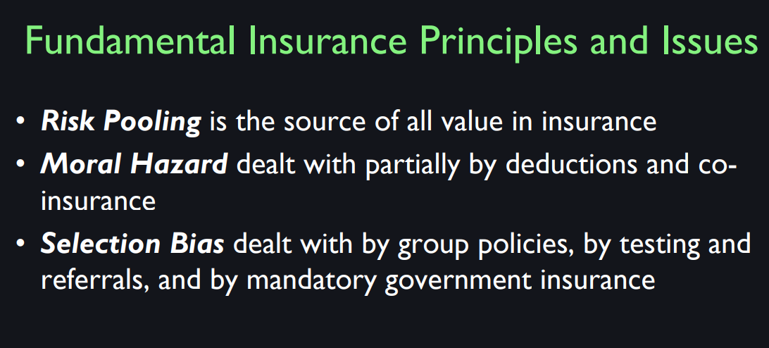
There is a theory behind insurance and this theory is risk pooling. That, what is a risk for one person is not a risk for society at large if they are independent. Because by the Law of Large Numbers, the number of bad outcomes are fairly predictable. The insurance company pools all these risks, and by the Law of Large Numbers is not really risky in itself. There’s a little mathematical formula for risk pooling which is assuming independence, if every, let’s say it’s a life insurance. If every death is independent of the other, there’s no epidemics or wars that bring a lot of deaths all at once. Then the risk that you face if you’re writing any policies each against one life is, the standard deviation is given by the √p(1-p)/n, where p, is the probability of death. And you can see that as n gets large, the standard deviation approaches zero. The fraction of policies that result in death becomes practically unknown number. That’s the key idea of insurance.
According to the Law of Large Numbers, the average of the results obtained from a large number of trials should be close to the expected value and will tend to become closer as more trials are performed. The Law of Large Numbers is important because it guarantees stable long-term results for the averages of some random events. So, let’s take an example. While a casino may lose money in a single spin of the roulette wheel, its earnings will tend towards a predictable percentage over a large number of spins. That’s how the casino can confidently pay its monthly bills.
Another example would be, if we took a six-sided dice and rolled it many times, the average of their values sometimes called the sample mean is likely to be close to 3.5 with the precision increasing as more dice are rolled. Unfortunately, it’s not so easy to make this idea work in practice, largely because of moral hazard and selection bias. Moral hazard occurs when people knowing they are insured take more risks. So for example, if your house is insured against fire you may say, “I don’t care, I’ll be careless with fire because it’s insured.” So then the risk goes up. Or even worse, if the insurance company insures your house for more than you think you can sell it, you would say, “I’ll just burn it down and pretend it was an accident. And then I’ll get more money than I would have for selling the house.”
Selection bias is different. It is that, the insurance company may not be able to see all of the risk parameters that define risk then their customers may see them more. So for example, health insurance tends to attract sick people. So health insurance companies ask for a medical exam, traditionally, to screen out people who know they’re already going to be sick. If they’re not successful in doing that, then the selection bias can harm their business and it can destroy an insurance business because, if people know that they’re going to be sick, then only sick people sign up. The insurance has to be expensive. Healthy people won’t sign up because they don’t want to pay the expense and so the whole thing collapses and doesn’t work. So you have to deal with selection bias the best you can by exams and disclosure and also by mandatory. The government can make it mandatory that insurance companies do not look at the selection. Obamacare is known for that, that health insurance companies are not allowed to take preexisting conditions into account.
Let me give you an example of moral hazard and selection bias in insurance. Many people in this world today are living in marginal economies, subsistence farmers. You have a farm in some very underdeveloped part of the world and you depend on the crop every year to feed your family. But unfortunately, the weather throws up those curveballs every now and then. There will be a typhoon or there will be a drought of some sort. So farmers should buy insurance, right? But, how do we do that? One kind of insurance that’s been offered for many centuries, I suppose, is crop insurance. So the farmer buys insurance against the crop failing. That sounds good and workable.
There’s a problem with it though. The problem is that it’s subject to manipulation. The farmer can lie about the crop, right? He can say, “I didn’t get much of a yield this year.” He can sneak some of it off and sell it and then try to claim on the insurance. Or the farmer can just get careless. Maybe he’s just not that focused guy, right. He doesn’t do things right. He gets drunk and he doesn’t do the necessary thing. That’s a moral hazard.
And then there is selection bias. Farmers who know that they’re living on marginal land will be the ones who will go for the insurance. So, crop insurance has been around but it hasn’t worked that well. This leads to an advance that occurred in the last 20 years or so as pushed by the World Bank, which is an international development institution. How about insuring the weather instead of the crop? Okay, because the farmer can’t cheat on the weather. He can’t make bad weather. We have weather stations. So that sounds like a good idea? Well it’s a new idea. Weather insurance for farmers. And it’s starting to catch on especially in the developing world where it’s extremely important. It can be life or death for some of these farmers. But then, does that sound obvious and workable? Can you think of any problems with weather insurance? You have to define the weather very carefully if you’re going to describe the effect on crops. It turns out that, if you plant seeds on a certain date and they start germinating they’re very vulnerable to drought. After a certain number of days after planting and if the bad weather comes right then, so you have to measure it locally and know exactly when the planting was, details like that to make it work.
Along the lines of moral hazard Jason mentioned, you cited an article that says that we are transforming from financial capitalism into more like philanthropy capitalism, and my question is do you think that the increasing number of philanthropists and NGOs causes people in the developing countries to have less of an incentive to insure these natural disasters? Okay.
That’s a complicated question. The reason we want insurance as opposed to gift giving is because insurance is much more logical and priced out so we know exactly what cost and what you can expect. And so for example, flood insurance in this country was created to prevent people from making big mistakes. The big mistake that was being made was that a lot of people were building houses in flood plains and you know sometime in the next 20 years, it’s going to be a big flood. And then these people are apparently counting on. “Well, someone will bail me out.” So in the United States in 1968, Congress passed a National Flood Insurance Act which specified that you had better buy flood insurance and the government will subsidize it but it will be priced appropriately. So go ahead, build your house in a floodplain but you’re going to have a sky high insurance rate. We’re going to price it out. And that’s the idea. So people are forewarned. You better watch out because this is a high risk area and the flood insurance rates will tell you that. So that’s a coherent system. If it’s just philanthropy, then people would always…a lot of people would be building on a flood plain. So, you’ve got to have it priced out and done right.
Insurance Milestones
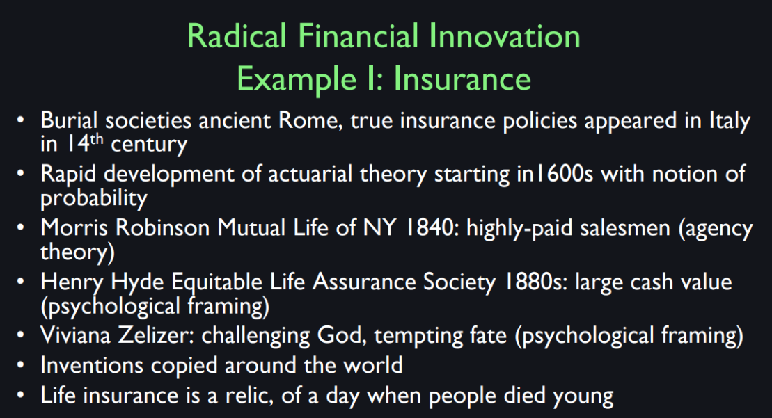
So, in order to make insurance work it takes a lot of developments and it’s not easy and obvious. The concept of insurance, as we pointed out, goes back to ancient Rome but it doesn’t seem to have taken over. It wasn’t managing most risk. It was a narrow scope of risk.
If you look at the history of insurance, insurance developed because of specific technical advances like the development of actuarial theory. So it was in the 1600’s that they produced the first life tables. And what they were, it showed the probability of dying at each age. That’s what you need to know if you’re doing a life insurance policy. What is the probability that the insured will die? And they didn’t, nobody had any statistics anywhere in the world on that until the 1600’s. So they started doing life insurance but it didn’t take off well. And fire insurance, it wasn’t widely accepted. The people mistrusted it and didn’t understand it. Even in my family, my grandfather who owned a farm in Michigan, lost their house to a fire and they weren’t insured. So this is part of our family. My family moved into the chicken coop, lived there, because they came home one day, they were on an outing and they came home and the house was gone. It completely burned down when nobody was there.
So there are some milestones in insurance history about how we can get things going so that it works. In 1840, Morris Robinson who is the head of the Mutual Life of New York, a mutual insurance company, got the idea that what insurance company really needs is insurance salesman. And these had to be pillars of the community type people. And so they had to be paid very well. So the idea it was, he was going around hiring exemplary men, I assume they were all men in those days, and he had to make a door to door call. It’s unusual you get a man that looked like someone you’d heard of as a pillar of the community coming to your house. Maybe they would do it through your church or somehow get introduced. But you needed salesmen because people resisted the idea of paying for something like insurance which seems abstract and you can easily forget the risks. It turned out that you had to pay these guys a lot. They had to keep coming back and re-affirming. They had to pay another visit to you because you would tend to stop paying on the insurance after some years when you hadn’t had a claim.
Then Henry Hyde in the 1880’s discovered having the sales appeal of having insurance with a large cash value. So, if you stop paying your insurance, you lose the cash value. And it’s also a saving vehicle as well. Why combine insurance with savings? Well, because it seems to affect the psychology of the purchase. And Viviana Zelizer, who is a sociologist at Princeton, did a big study of how insurance was marketed in the 19th century. And she said that, talking particularly about life insurance, women were the main beneficiaries of life insurance because men were the breadwinners, are earning an income and they tended to die young in those days. But women seemed to be, according to her studies, objecting to life insurance saying, “No, I don’t want that.” So why would a woman say that in the 19th century? Well, partly because Viviana Zelizer concludes, they were Fundamentalist Christians and they believed in the power of prayer. And they thought, women thought that insurance was some crazy gimmick scheme. And they wanted to trust in the Lord rather than in some thing that looked like gambling. So one woman said, apparently, “You know, this insurance policy it looks like I’m making a bet that my husband will die.” And she said that will encourage God’s wrath. I should stay out of that because I’m challenging God to take my husband and I should not do that.
So they developed a different sales pitch and the new sales pitch was, don’t try to explain probability theory. Don’t try to explain how this business works. You come to the wife and you tell her, “I have a mission, okay. My mission is to help your husband protect you from beyond the grave. If God forbid something horrible were to happen to your husband, you know he would love and protect you if he could. I’m making it possible.” And that, that seemed to work and women went along with it. So these are, these are little inventions, they’re marketing inventions, but they’re important. Now we don’t need life insurance as much because people live longer. Really life insurance is to protect families against the death of a father or mother while young.
Advantage of insurance might be that it has an information value that, if like you were saying earlier, if I look up the growing premium on an insurance for insuring some flood on the other side of the country, then, I look at the price. It is going up, then all of a sudden i’m inferring something [inaudible]. Right. The risk in that area without even having visited - Right. So that has other [inaudible]? Yeah. If they didn’t have the insurance then the seller of the property has no incentive to tell you about the flood that we had 20 years ago. You know you can’t see the damage anymore so you might not know, there’s no incentive. But if, if, if you are looking to buy insurance and then you see they want a thousand dollars a month for insurance, what are we talking about here? This is crazy. Why is that? Then, yeah it makes an impression on people. You know, I talk a lot about human psychology and human failures but there is a certain element of rationality and that moment happens when you’re about to sign the papers for your insurance and you say, “Wait a minute.You want me to pay a thousand dollars a month just for the flood insurance add on?” Then it makes you think and most people will make somewhat rational response to that.
Insurance is a Local Phenomenon
Insurance is a complicated
thing because it has been regulated for centuries and
it’s often regulated at the local level. In the United States insurance
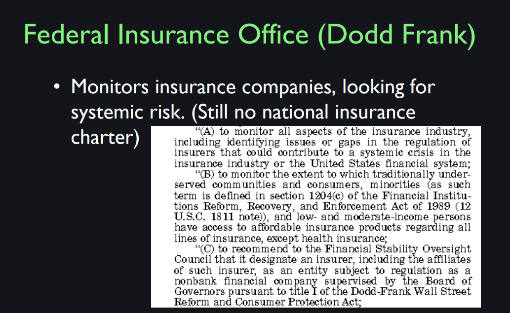
is a really local phenomenon. The Dodd Frank Act of 2010 created
a federal insurance office. But it’s really mainly just
a monitoring for risk. There are no national insurance companies,
they all have state charters. Also, what protects you if your
insurance company goes under? Well, the regulator is supposed to have
checked that they’re doing things right.
But what if the regulator messes up and
you buy insurance? And now there’s some big catastrophe and
the insurance company goes bankrupt and can’t pay you. So the state governments have set
up insurance guarantee funds. There’s a lot of complexity
to this whole business. It’s not so simple and easy. So the first step, it wasn’t until
the 20th century that these even setup. It’s like deposit insurance
when you have a bank. When you go to the bank, you’ll see FDIC insured, Federal Deposit,
Insurance Corporation, but we have similar insurance of
the failure of the insurance companies.
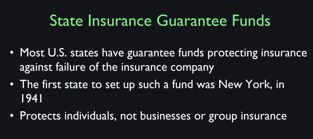
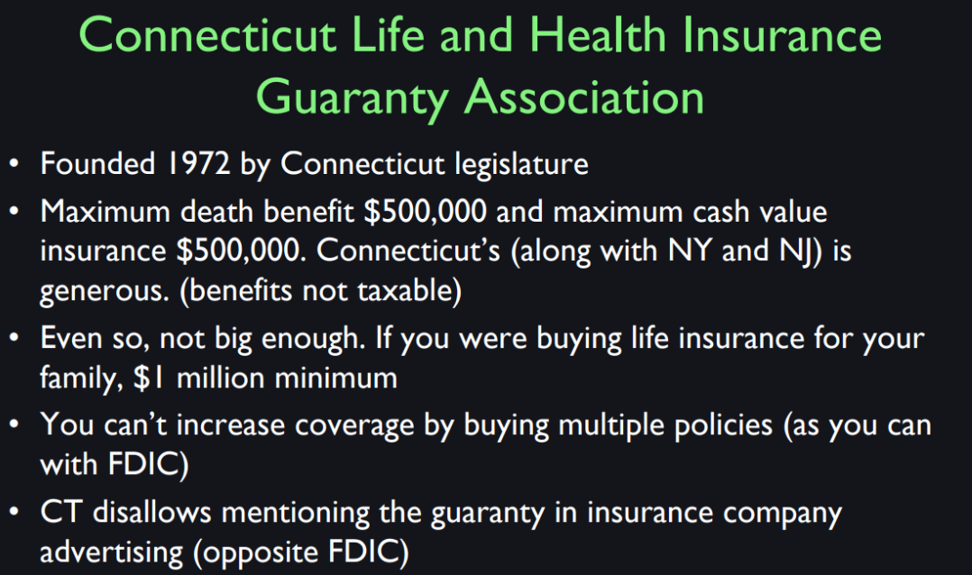
But not until 1941. There was no insurance guarantee. So, here’s our local insurance
guarantee fund, Connecticut Life and Health Insurance Guaranty Association. It was created in 1972,
it’s not, that long ago. It’s kind of remarkable, that before
1972 if your insurance company failed in Connecticut you were just out of luck. But now they will ensure
your insurance against a maximum death benefit of $50,000. It’s still not big enough because
if you as a young person, what is your present value,
your lifetime present value? It must be several million dollars. So $500,000 just doesn’t cut it,
but at least it’s something.
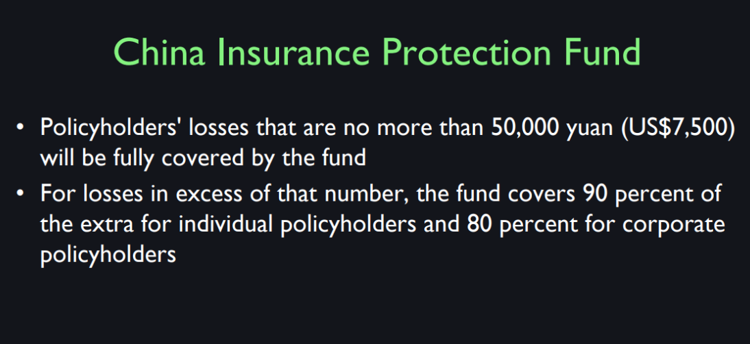
Other countries have insurance. The China Insurance Regulatory Commission
has set up a state-owned non-profit called
China Insurance Protection Fund that protects people against
the failure of an insurance company. But again, they’re limited to 50,000 yuan,
which is not much money. So we still live in a world that’s highly,
you gotta watch what you get into and check things. One thing I like,
this is a course in financial markets, and I like this institutional detail because
to me, it’s what makes things work.
So, when you’re talking
about AIG the last lecture and how they take the whole government
bailout, what’s preventing them from committing their own moral
suspicion of moral dubiousness. If they know hat there’s something
like a big catastrophes coming again, they’ll get another bail
out because they’re so big. Are there regulations im place? >> Well the financial crisis of
2008 took everyone by surprise. The bailouts weren’t
the planned course of action. It just happened. It got so severe so
suddenly that the government stepped in. In the US and in other countries to protect the
integrity of the whole financial system. Now the issue now is does this set
a precedent that insurance companies will say, hey we don’t need reserves
because we’ll just get bailed out. Well that’s a concern and
it’s been a concern of law makers. Part of the issue though is
that AIG was bailed out but the stock holders did not do well. They didn’t enrich the stock holders. It was a disaster. On top of that I think that our
new regulations are stiffer and and are more aware of that crisis, but you are getting at a really important problem
that too big fail is a natural problem. When you have a complicated
interdependent economic system and if one big company like AIG fails, that was the
biggest insurance company in the world. Once one company like that fails, the government isn’t wanted to just
let it everything fall where it may. There’s a natural tendency to bail out and
it’s hard to get past that. We’re making efforts to, but
it’s a fundamental problem.
The US Government took
over securities regulation in the 1930s after the Great Depression. They formed the Securities and
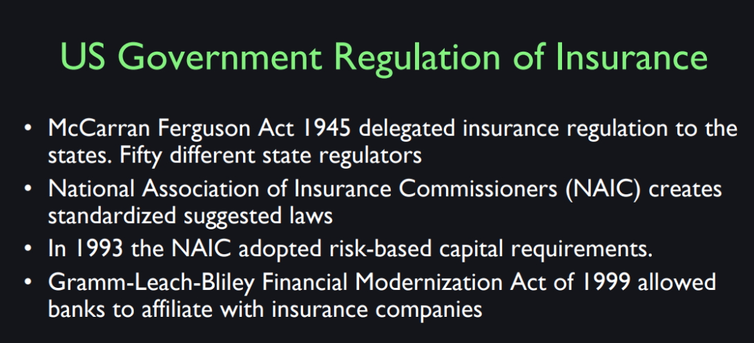
Exchange Commission to regulate stocks and bonds from the federal level. They never did that for insurance. In fact the McCarran-Ferguson Act
of 1945 delegated insurance regulation to the states. So there’s 50 different state regulators,
all different. Now this is chaos, because companies
like to operate nationally, but they have 50 different regulators,
one for each state. So there was a non-profit called National
Association of Insurance Commissioners, NAIC, which is not government. It’s set up by the insurance industry and they have regular meetings creating
suggested laws for insurance. That helps reduce the complexity
of the US insurance system, because at least the state
governments talk with each other, and standardize their insurance laws somewhat.
Health Insurance
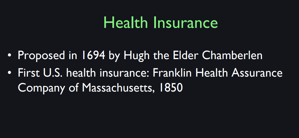
Okay, the first health insurance, apparently was in 1694. The first U.S. health insurance company was Franklin health insurance company of Massachusetts in 1850.
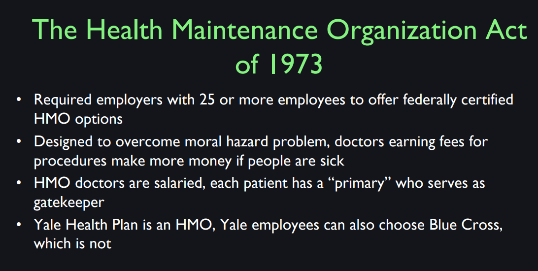
There was an important step forward in health, in Health insurance with the health maintenance organization Act of 1973 which required employers with 25 or more employees to offer what’s called an HMO. A health maintenance organization. The idea at that time was that the medical services were generally provided by practitioners, to uninsured people who had to pay when they were sick. The problem was that doctors made more money if people were sick. They would, they didn’t have any incentive to prevent disease. So there were people who complained that we needed to have our our health managed by practitioners who had an incentive to keep you healthy to do preventive things. So how do we do that we have to create an organization like the Yale health plan, that keeps you for a lifetime. Let’s say that gives regular checkups to you and encourages you to come and talk to the doctor. The doctor has no incentive because a doctor is paid a salary, has no incentive to urge unnecessary surgery on you or the like. So this is what Yale health plan which was a pioneer. It was one of the first HMO’s. What they do at, I think you’ve been there right. They assigned you a primary, which is the gatekeeper for you. And they encourage you to come in for any minor thing which might reveal a more serious problem.
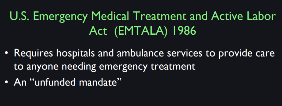
In 1986, the U.S. Congress passed another law called EMTALA law. Emergency Medical Treatment and Active Labor Act which required hospitals and ambulance services to provide care to anyone needing emergency treatment. So basically it was a tax on everybody to provide emergency services. Now, you could probably go to an emergency room before 1986 because there was some, public spirit that hospitals would treat you if you came in. But it became mandatory in 1986. But it’s not the same thing as health insurance. Because they kind of hope that you take your sick people to another hospital’s emergency room not ours, because it comes out of our pocket, if you can’t pay. So it’s not a… it is a not a great system. Then it came, as you’ve heard of the U.S. Pain Patient Protection and Affordable Care Act of 2010 called Obamacare. And it tries to deal with the selection bias problem by forcing everyone to sign up. So there’s a penalty for individuals not buying insurance. A tax penalty. And a penalty for companies not offering insurance for their employees. So they set up health exchanges that try to regularize the competition among insurance companies. It’s a complicated system that the Republicans want to shut down, as soon as possible. But to me, Obamacare reflects some really important issues in insurance namely that the U.S. has had something like 45 million people uninsured. And if they are uninsured then they will go to the emergency room when they are dying but they don’t. It’s not a good system because they don’t get preventive care and they don’t, they only end up In the last stage of collapse at the medical system. So it’s not perfect.
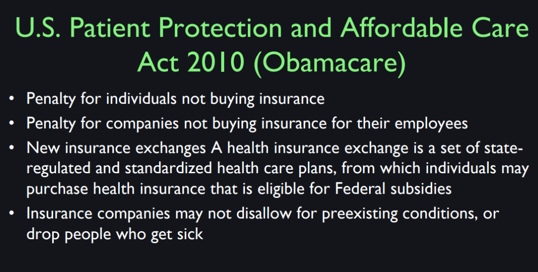
Earlier when you were talking about mandatory health insurance, now that Obamacare is kind of pushing into the direction in the area of health insurance, do you think that’s the Right thing? Right. Well see. Health insurance has suffered an important shortcoming in the United States. It’s not, hasn’t been offered by the government. It’s private, and it’s often through employers. So suppose you lose your job then you’ve got to go out and buy health insurance. Now the problem is that they will look at you, and if you are sick they’ll say will charge you a very high rate. And so and they also have a selection bias. We talked about this in class that the people who sign up for insurance are the people who know they’re sick and need it. So that means you have to charge very high rates and then people who know they’re healthy will not sign up because they don’t want to pay the high rate. So nobody is insured, or not many people are insured.
So the Obama, the Obama Care Act in Congress made it mandatory. You would pay a fine if you don’t sign up for insurance. That was supposed to put everyone back into a pool where everyone is insured and was supposed to bring the rates down. So you have to do something like that this, this is the fundamental problem with insurance. If if it’s not a risk it doesn’t work. If people know there that they are at special risk then it’s… it’s not going to work. You can only insure against the unknown, but you can make laws that prevent companies from taking account of, of risk factors so that people can buy insurance and that’s what Obama here did.
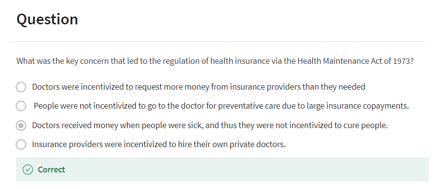
Disasters
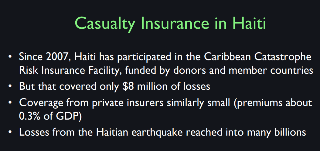
Most people in the world do not have
insurance against earthquake risk. Now that seems almost astonishing
because the risk is so well quantified and there’s such
an incentive to manage the risk. So this is a picture from
the Haitian Earthquake of 2010. And you can see the damage it caused and yet most people there were not insured. So the earthquake came in 2010,
before the earthquake there was the movement that tried to get
Caribbean countries to buy insurance. And so they did so only a little bit. The Caribbean catastrophe
risk insurance facility, manage to a create about $8
million of loss insurance. [LAUGH] But the loss is from Haitian
earthquake reached into the billions. So why weren’t the Haitians insured? There was an organization
trying to get them to do it and they could have bought it. But apparently, there was a resistance
a thought that maybe a mistrust of institutions, a tendency to believe
in good luck or something like that.
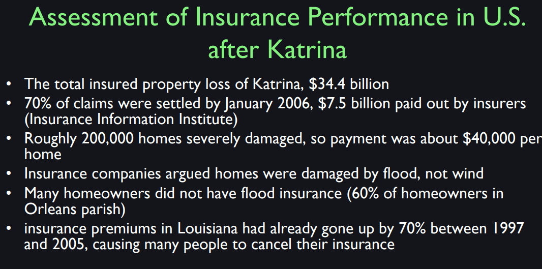
Here’s another example. Hurricane Katrina is 2005. Now, this is in the United States where
people are much more sophisticated, I would say, or
at least attuned to financial solutions. So the city of New Orleans
was heavily damaged in the Katrina hurricane. But again if insurance wasn’t
perfect there as well. So now this is totally
different from Haiti because we have a lot of insurance
in the United States. There was in fact losses of $34
billion caused by the hurricane. And these were settled and paid out. But there were problems then, again, the problem was that a lot of
the insurance policies were insured against wind damage,
but not flood damage.
Now, before the fact,
when you sign the insurance contract, this might seem like a minor distinction. Because Hurricane Katrina
was both wind and flood. But many of them did not
have flood insurance. Now why didn’t they? Maybe they couldn’t imagine how
can it flood here in New Orleans? They didn’t understand the impact
that a hurricane can have. So also maybe because of global warming
and greater fears of hurricanes, the insurance companies had been raising
their rates on hurricane insurance. So many people in New Orleans had cancelled their insurance because
they thought it got too expensive. So there was this substantial failure to
compensate people in New Orleans as well. Not as bad as Haiti.
You’re saying why should I buy flood
insurance if I just say I didn’t do it sorry I’m I’ve made a mistake
someone will come and help me. And so I’m going to build the house on
a flood plain anyway because I don’t care. Now, that was a problem. When they passed
the National Flood Insurance Act in 1968, people didn’t just go and buy it. They were ignoring it. So one thing that, later,
Congress, in 1973, passed another act that
made it mandatory to buy. It wasn’t a choice anymore. You had to buy the insurance. If you were building in what was
a designated high-risk area. On top of that,
the US government has tried to tell you, we are not going to help you that much. If you didn’t buy in areas where it
wasn’t mandatory, if you didn’t buy flood insurance, the government will
limit their help to loans. So okay,
you’re house was washed away in a flood. You didn’t buy flood insurance. Well, we’re not going to
just forget about you, we are going to lend you
the money to build another house. So the government is there but
it’s not helping you that much. So they’re trying to create a system
with the right incentives and the bottom line is,
stop building in flood prone areas. And if you do make the mistake,
you will only get minimal help. And you better know that
when you build a house. Some people disregard everything. I’m sure it’s still happening, but
it’s kept down to a small number. I think this is one of
the wonders of modern capitalism that we do as well as we do.
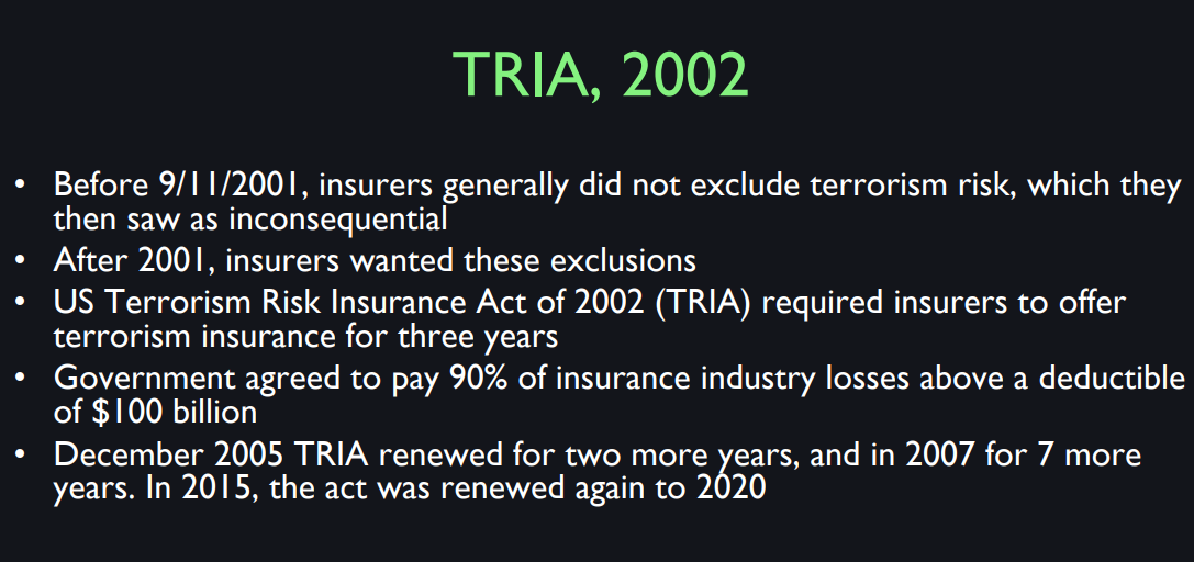
And then finally we want to
talk about terrorism risks. Insurance policies have in the past
generally not focused on terrorism risk. Before 9/11/2001, most insurers did not exclude terrorism risk because they
didn’t think that it was even a risk. But after 2001, they started changing their policies
to say we don’t cover terrorism. This led to a sense of frustration
that this is a big risk that people are suddenly concerned about,
and they can’t by insurance against it. For the insurance company, said that
this isn’t the way we do business. We don’t insurance against
correlated risks like that. There could be a huge terrorist attack,
and how do you expect us to pay it out? In this case,
this is an example where the government plausibly becomes involved and
has been involved in history as well in providing
the insurance against the acts of war. Because the insurance companies
can’t do it by themselves.
So in 2002, the United States Congress
passed the TRIA, the Terrorism Risk Insurance Act of 2002,
which required insurers to offer terrorism insurance for
three years. But the government would pay for
it, or at least 90% of it. Because they decided it was too much
of a tax on the insurance company, to asked them to bear this risk. And what were they charged for? That’s the thing because they
don’t know where it’s going. So the government agreed to pay 90% of the insurance industry
losses above a $100 billion. So that act keeps expiring and
keeps being renewed again. So by 2015 the act was
renewed again until 2020. But you think they should just
make it permanent, right? Why is it a temporary thing?
It reminds me of bankruptcy law. In the 19th century, if you went bankrupt,
let’s go back to 1800. If you couldn’t pay your bills in 1800, they had special prisons for
you called debtor’s prisons. But there were repeated financial
crises through the 19th century. And, A lot of people went to debtor’s
prison who were perfectly innocent. The only crime they’re guilty of is not
understanding that they would lose their job in a financial crisis and
they couldn’t pay. And their company would say,
it’s something like that. It’s not really their fault. It’s not something we
want to see punished by jail. So in the 19th century, whenever there
was a financial crisis, they passed some special bankruptcy law that had a time
duration like this and expired. They thought, well, we’re just
dealing with the current crisis. But as time went on,
these crises kept coming and eventually, bankruptcy law became a permanent fixture,
not just a reaction to a crisis. So that’s probably what should
happen to TRIA eventually. There are certain things
that are hard to insure. And we require the government
to come in to do the job. We’ll come back to that when we
talk about public finance later.
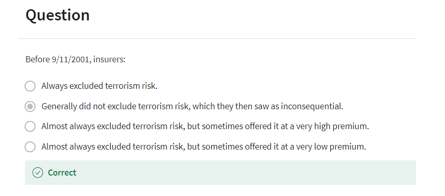
Generally did not exclude terrorism risk, which they then saw as inconsequential. 一般不排除恐怖主义风险,他们当时认为这种风险无关紧要。
Lession #3 Quiz
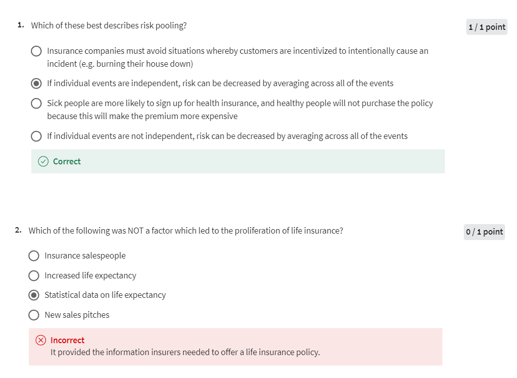
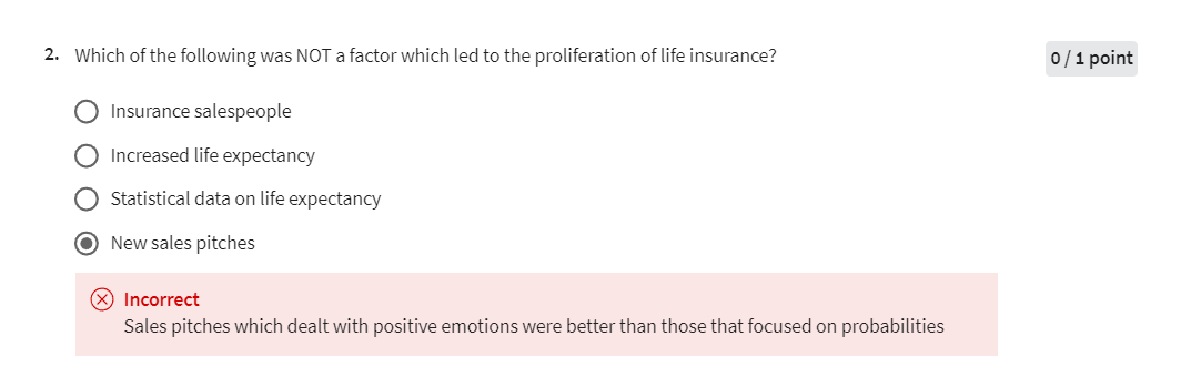
第二题正确选项如下:
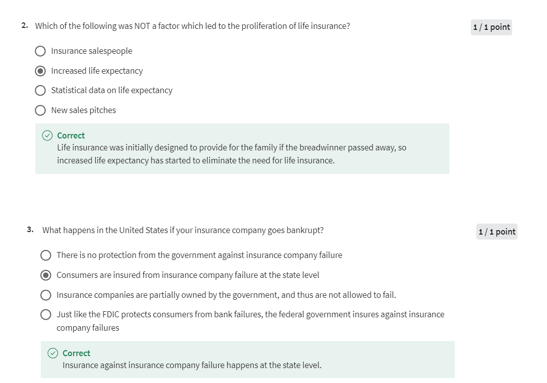
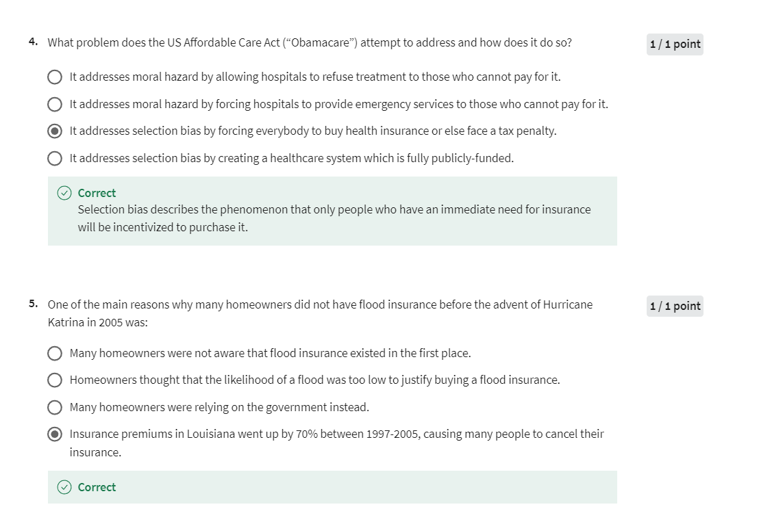
Lesson 4
Eggs in One Basket
And I wanted to talk about
an alternative to insurance. It’s the idea of managing
risk not through purchasing an insurance policy, but
through diversification. Through owning a variety of assets. And here again, we’re going to
start by assuming a blank slate. You as an individual have no
risks that are inherent to you. You don’t live in an earthquake zone. We’re not going to worry about that. But you do have to take on risks
in order to get a good investment. So the idea is that risk
is inherent to investing. You can’t, ultimately, people who
are providing you with investment opportunities are doing something
in the real world, which is risky. And if it weren’t risky,
it wouldn’t be giving you an extra return. That’s the core idea
that we want to develop. And that you have to manage your risk by
diversifying across a number of different assets, not putting all
your eggs in one basket. So that’s the core idea that
we want to develop today.
So I said, put your eggs in one basket. I was wondering, you’ve heard that term. Don’t put all your eggs in one basket. That’s a very [INAUDIBLE]. Who said put all your eggs in one
basket and watch that basket. That might have been Mark Twain. I have to look it up. But, more famous is don’t put
all your eggs in one basket. So, I tried to search where
did that first appear? And I found it in a book by Alexander
Crump in 1874 about how to invest. And then he says, there is an old saying. [LAUGH] That it is inadvisable to
have all your eggs in one basket. So he doesn’t provide a reference for his old saying but that’s the earliest
reference I could find for it. I like history of thought. I always wonder where it comes from.
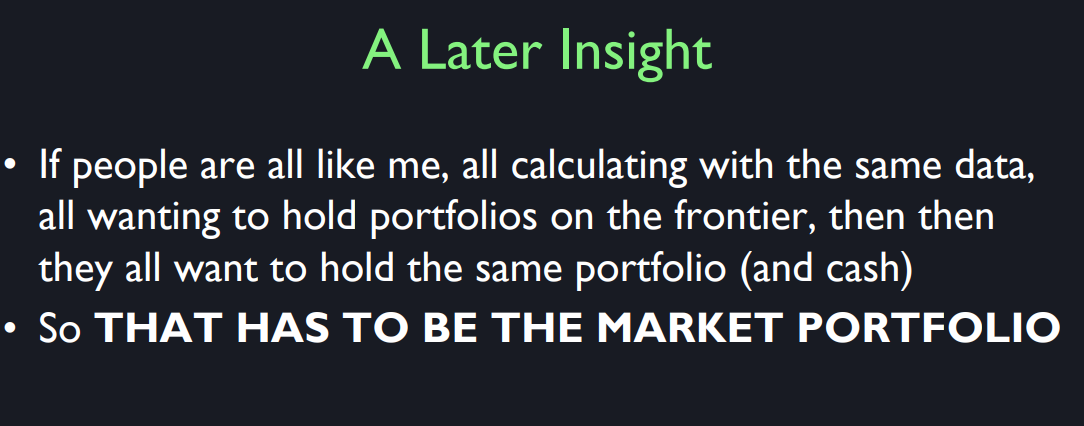
The portfolio theory approach
describes everyone as the same. We don’t, we don’t have risks
that have to be insured or we’ve already taken care of them. Any specific risk. I bought an insurance policy. And it’s gone. So, that’s the assumption. So, what if I calculate the optimal
portfolio, the best diversified portfolio? The insight, the core insight of
this theory is, you know what? It’s going to be the same for everybody. I mean if I can serve quantified risks and
returns and I calculate the optimum. Then why is it different
from one person to another? Well, you could be different
from another person because you might be more
risk averse than others. You might have a greater or
lesser tolerance for risk. But that variation and tolerance to risk could be adjusted by
leveraging your portfolio up and down. So if you abstract from that adjustment,
really, everyone should be doing the same thing. That’s the key insight. So all that should matter to you as an individual is the performance
of your whole portfolio, right? If you’re a rational, economic person, an econ as they call them, why do you
care if one stock goes up or down? It’s the total that matters to you. So, what you would naturally
care about is the mean and variance of the return
on your whole portfolio. And you just don’t care about
what one asset or another does. Now, in fact, people boast about their investing
skill with regard to individual assets. But they shouldn’t because you
win some and you lose some. It is the average that matters. So you care about the average
return of your total portfolio, and you care about how uncertain the total
return of the whole portfolio is.
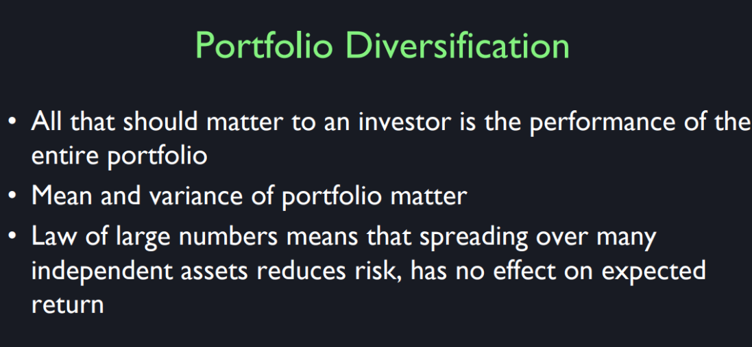
We are talking now about
the capital asset pricing model, which I think, it’s due to
Harry Markowitz, in the early 1950s. He was a graduate student
at University of Chicago. He had this neat idea. I can write down how to optimize risk? I’ll assume risk can be
described by a variance matrix, a little bit of technical apparatus,
and statistics. And I suppose I know what the expected
returns are in various assets. What should I do as a portfolio manager? And it was simple. It was like one page of math. He wrote it all down. Computed the optimal portfolio. And assuming that you know the variability of assets and their expected returns, it kind of amazes me that
It wasn’t known before. But there are moments in history when
certain ideas suddenly crystallize. The idea of measuring risk
by a standard deviation. And then doing some calculations that
bring that down maybe to a minimum value or minimum compared to
some expected return. That led to a big revolution in finance.
So, but it’s a mathematical discipline,
not that we saw in class. I also think it can be overrated,
I love mathematical models like that, but they’re not the whole story either. But the idea is that somehow
you have to take account of each asset that you invest in. How does it contribute to your
overall portfolio variance and portfolio expected return? And there’s a lot of
complexity in the decision. Sometimes you want to be hold
the positive amount of an asset, sometimes you want to
hold a negative amount. And what you hold depends not just
on that asset’s expected return, but on the expected return of other assets and
their covariance with this asset. It all sounds impossibly
difficult problem, but it really isn’t that difficult. It’s simple calculus. Harry Markowitz just worked it out in his
room at the university City of Chicago. And it’s with us ever since. So that was one thing I wanted
to cover early in the course. because I just like the model. I don’t trust it either [LAUGH] but
I like it.
Salon - Risk
Think of risk, I was wondering how these
large hedge funds and their ability to take on large amounts of risk and leverage
themselves, how that affects the market? >> Well hedge funds
are investment companies that are not approved for
the general retail market. So they’re not allowed to advertise. They’re not well-known, because they’re
not allowed to promote themselves, except through private conversations,
and to invest in them you have to be an accredited investor,
not a general investor. So they are allowed to do
sophisticated and dangerous things. The idea is a hedge fund is regulated for people who have professional advisors or
family offices. You know what a family office is? If you are really rich you
don’t just hire an advisor. You get a team of advisers, who that’s their whole job,
is to work on your family investments. That’s what hedge funds are really for. So they’re dangerous because they’re not, it’s like taking drugs. [LAUGH] You need a physician to,
between you and the drugs. Then, so often in the past hedge
funds have done really well. In recent years, they haven’t been doing
well, on average, for the most of them. So I don’t know that I recommend them. I can’t recommend them as a group. But if you’re,
do you have a family office? [LAUGH] I assume you don’t. >> Unfortunately I do not.
[LAUGH] >> If your family office recommends it, go for it,
if you’ve selected them carefully. But they just represent claiming to
be the most sophisticated investors. Another notable thing about hedge funds,
is that traditionally they pay very high rewards to their investments
managers if they out perform. But that comes out of your pocket. And there are skeptics of hedge fund
saying, I would never pay those high management, those expenses,
to the people who invest my money. Because nobody can deserve that amount,
and so hedge funds in a sense are, at least many of them,
have been a bubble in themselves. They were doing well for awhile. The impression was that they were doing
well, lots of people piled into them, and lately they haven’t been doing so
well.
I guess really that these big financial
institutions, can take on a lot of risk, and this risk that they take on has a
potential to cause mass financial crises. Should there be a way to
regulate this risk or how much of this risk should be
regulated versus how much is it important to the inherent way that
these institutions are working? >> Yeah, well, I think that we
are in a situation where we had heightened recognition of
the importance of regulating for dealing with big risks that,
systemic risk. So a systemic risk is a risk that
the whole system will collapse, like a house of cards, some people say. Regulation before 2008-2009 crisis, was mostly micro-credential. That means they wanted to make sure
that you as an investor weren’t being ripped off by this stockbroker
who was squirreling away your money or doing something like that. They were thinking of
you as an individual. But we’ve now had new impetus for
macro-credential regulation, and it’s now regulation about how
interconnected are you with other, or some big business connected, and what will happen if that other
business fails to this business? So we want to, or if there’s a world financial crisis,
how will this business fare? So, since the 2008-2009 financial crisis, we 've seen a lot more
macro-credential regulation and a lot more measures of risk
that are being developed. There are now what we call
stress tests of financial institutions that emphasize more
on their interconnectedness, and how they would act, how they would fair
in various kinds of international crisis.
What are some measure of risk,
I guess, post 2008 crisis now, that are more appropriate to measuring? >> How accurate are these measures? >> Yeah, well there’s a,
that’s a controversy. Before the crisis,
there was regulation, it’s not new, and there was some concern
with macroprudential. For example, before the crisis,
there was a method called value at risk, that was used
to measure the risk of a company. By looking at the assets and
liabilities of the company and considering what the probability of big direction in the values would be and
what it would mean for the company. But after the financial crisis we now have
more elaborate assessments of macro risk, and the stress tests will consider,
well the government regulator will specify that the financial
institution should estimate how it would be affected by
various kinds of financial crises. So, it’s getting more detailed, and
more effort is being put into it. That’s because the 2008 crisis
caught us all off guard, and people just didn’t know
how interconnected banks, and other financial institutions were, and
they had to act in ignorance as a guess. Because their, too much of their data
collection was micro-credential.
I have one more question. >> Yeah. >> It’s about going back to the ideal of
measuring risks so in class you mentioned, Nassim Taleb’s idea of the Black Swans. And he said that all these models to
measure risk are, if you read his book, are fundamentally flawed because they
don’t take into account this super run like improbable events. >> Right, right.
Where you consider the financial crisis into the [INAUDIBLE] was
one of those events. So do you think there’s ways to improve
this model to take into account more unlikely events that this platforms,-
Yeah. >> The method is fundamentally
flawed to take into account. >> Right.
So you’re referring to Nassim Taleb, who had a book called the Black Swan,
that talked about rare, low-probably events as
being sometimes really big. >> Yeah. >> So you can work a lifetime creating a, creating wealth under certain assumptions
that something can’t happen and then bang. Everything, you’ve lost everything for your whole lifetime,
because you thought it couldn’t happen. That’s kind of what happened
in the recent crisis, people thought that home prices can
never fall, because they never have or they never have since
the Great Depression [LAUGH] and so- >> [INAUDIBLE] >> I know that’s a perfect example, but this it’s how to deal with academically. If you’re talking about rare, big events, well you don’t have enough data
on them because they’re rare. So, it’s a problem. So, things that happen in the market, this
is what efficient market people sometimes say, that the markets have to deal with
the probability of these rare big events. But they are so intangible and they
are just something that i can’t quantify. But when the market goes down,
Eugene Farmer might say [LAUGH], when the market goes down,
don’t just assume it’s crazy. Maybe it is some subtle evidence about
some big event that could happen. So I gotta give it,
that is a possible interpretation. We just never know. I wish there weren’t these
big black swan events, finance would be so
much better a [LAUGH] profession to be in. Unfortunately, we live in a real world. [LAUGH] I shouldn’t put it like that. >> [LAUGH]
We live in a world with the risk of huge events. >> So we have so many risks in our life,
like as we said, if you go into a labor
market during a recession. Or basically, if something bad happens,
like you need to find a way to hedge it, we have stuff for, like hedging
against oil risk or agricultural risk. Are there any innovative
financial products for hedging against the labor market risks?
I’m glad you asked that question
[LAUGH] because this has been a theme of mine for a long time,
that we should have labor market risk. Now we do have something. Unemployment insurance was started in
the United Kingdom, I think it was 1911. The idea is temporary assistance for
finding a good job. Now they realized, they’re in the UK, that people often are desperate
when they lose their job. They have a family, and
often people no savings. So what the person does is takes,
has to, take the first job offer, and it’s often not a very good
career track for them, and so it’s hard for them to move to another job. So, let’s give them time, let’s give them
may be six months of support so that they can find the right job, and also give
them some kind of help in finding a job. They will have a career service for them. That’s an old idea. The question is whether we can do more. The unemployment insurance is really
focused on finding a job in the short run. But now there’s a problem that we’re
seeing inequality grow in many places around the world, and we see a lot
of people who are complaining differently, that often it occurs
when they’re middle age, say they’re 50 years old and
they lose their job. They suddenly find themselves,
I mean they can get some job, but they can only get those bad jobs. Somehow people want to hire young people
and they’d have to be retrained, and someone doesn’t want to retrain them,
because right now it stays long, and so they have a problem. So one idea,
I call it livelihood insurance, this is kind of a futuristic idea,
but this is not just, there is Larry and Robert another couple of the economists wrote
a paper about 15 years ago. For this similar idea,
they called it wage insurance. So their idea is when somebody
loses their job and has to take a job at a lower wage, they should be
able to collect on an insurance policy. Interestingly, President Obama
brought this idea up during his State of the Union address for 2016. So the President of the United States
appears behind this idea. Unfortunately, a lot of ideas
that President Obama has been behind don’t happen. >> [LAUGH]
But the other thought of it, he was proposing to be
some government insurance. I don’t see why it has to
be exclusively government. There could be private insurers or private markets that would help
protect people against loss of income. But I think it’s actually very important
now, more so than in the past, because of the rapid increase in
information technology on robotics, and the rapid globalization. So things can happen really
fast that make one’s investment in human capital obsolete. And absolutely, there should be
risk management devices for that. And the important thing,
as I’ve argued in my books, [LAUGH] is if you help people manage
risks, they will take more risks. That’s what we want. We want people, in their decisions about
their education, to do some risk-taking. Develop some specialty that
is at risk of being obsolete, but who knows, nobody knows. You’re taking a chance. Let’s encourage people to take chances.
Summary of the Lecture
This lecture focuses on risk management in finance, particularly addressing the roles and impacts of hedge funds, the necessity for regulation, and the challenge of measuring and mitigating systemic risks. It also discusses innovative ideas for hedging against labor market risks.
Key Points
Hedge Funds and Risk:
- Hedge funds are investment companies catering to accredited investors and are not marketed to the general public.
- They engage in sophisticated and high-risk strategies, often leveraging themselves heavily.
- Hedge funds have historically performed well but have faced challenges in recent years.
- High fees are charged by hedge funds, which can be a significant cost to investors.
Systemic Risk and Regulation:
- Systemic risk refers to the risk of collapse of the entire financial system, not just individual institutions.
- The 2008-2009 financial crisis highlighted the need for macroprudential regulation, focusing on the interconnectedness of financial institutions.
- Post-crisis regulations include stress tests that simulate various financial crises to assess the resilience of financial institutions.
Measuring Risk:
- Traditional methods like Value at Risk (VaR) have been used to measure risk but may not account for systemic risk adequately.
- Post-crisis approaches are more comprehensive, focusing on potential global impacts and interconnectedness.
- Nassim Taleb’s concept of “Black Swans” highlights the difficulty of accounting for rare but impactful events in risk models.
Hedging Against Labor Market Risks:
- Current tools like unemployment insurance provide temporary support but are insufficient for long-term career disruptions.
- Proposals for more comprehensive solutions, such as “livelihood insurance” or “wage insurance,” aim to provide income support when individuals face significant wage reductions due to job loss.
- Encouraging risk-taking in education and career choices through better risk management can lead to greater innovation and adaptability in the workforce.
在金融领域,“hedge” 指的是通过采取某些策略来减少或抵消风险,确保投资者在面对不确定性或潜在损失时能够获得一定程度的保护。
在 “Hedging Against Labor Market Risks” 这一背景下,“hedge” 的意思是通过金融工具或策略来减少或抵消劳动市场风险对个人收入和就业的影响。这种风险对冲的目的是保护个人在失业、工资下降或职业生涯中断等情况下的经济稳定性。
例如,“wage insurance” 或 “livelihood insurance” 这样的创新金融产品可以为失去工作或面临工资减少的人提供经济支持,使他们能够在不显著降低生活水平的情况下度过困难时期。这种对冲策略不仅有助于个人应对短期风险,还可以鼓励他们在职业选择上更加大胆,追求可能带来更高回报的机会。
Learning Points
Understanding Hedge Funds:
- Recognize the high-risk, high-reward nature of hedge funds and their impact on the market.
- Be aware of the high fees and the necessity for sophisticated investment strategies when considering hedge funds.
Importance of Regulation:
- Understand the shift from microprudential to macroprudential regulation post-2008 crisis.
- Recognize the role of stress tests and interconnectedness assessments in modern financial regulation.
Risk Measurement and Management:
- Acknowledge the limitations of traditional risk measurement tools like VaR.
- Appreciate the challenges posed by rare events (Black Swans) and the need for robust risk models.
Innovative Financial Products:
- Explore the concept of livelihood or wage insurance to hedge against long-term labor market risks.
- Understand the importance of supporting individuals in taking calculated risks in their careers through better risk management tools.
By addressing these points, the lecture provides a comprehensive understanding of risk management in modern finance, emphasizing both the technical aspects of measuring risk and the practical implications of managing it in a rapidly changing world.
hedge fund
对冲基金是一种私募基金,专门为高净值个人和机构投资者设计,旨在通过多种投资策略获取绝对回报,即无论市场状况如何都力争实现正回报。对冲基金具有高度的灵活性,可以在全球范围内投资于各种资产类别,包括股票、债券、商品、外汇和衍生品。以下是对冲基金的基本工作原理和常见策略:
基本工作原理
投资者募集资金: 对冲基金从高净值个人、家族办公室和机构投资者处募集资金。通常,这些投资者必须是“合格投资者”,即他们具备一定的财务实力和投资经验。
灵活的投资策略: 对冲基金使用多种投资策略,包括长短仓、市场中性、事件驱动、宏观策略等,以在不同的市场条件下寻找机会。
杠杆操作: 对冲基金常常使用杠杆,即借入资金进行投资,以放大潜在收益。这也增加了投资风险。
对冲风险: 虽然称为“对冲基金”,但并非所有对冲基金都进行对冲操作。然而,许多对冲基金会使用期权、期货和其他衍生品来对冲特定风险。
高费用结构: 对冲基金通常收取较高的管理费和绩效费。管理费一般为2%,绩效费一般为20%,即“2/20”结构。
锁定期和流动性限制: 对冲基金通常设有锁定期,要求投资者在一定时间内不得赎回投资,以便基金经理能够执行长期策略。此外,赎回通常需要提前通知。
常见策略
长短仓策略(Long/Short Equity): 通过持有看涨的股票(做多)和看跌的股票(做空),基金经理希望通过个股选择和市场波动获利。
市场中性策略(Market Neutral): 通过同时持有等量的多头和空头头寸,基金试图消除市场风险,仅依靠选股能力获取收益。
事件驱动策略(Event-Driven): 利用企业并购、重组、破产等特定事件中的机会进行投资。
宏观策略(Global Macro): 基于对全球经济和政治形势的宏观分析,进行货币、利率、股票和商品等多市场、多资产类别的投资。
量化策略(Quantitative): 使用数学模型和算法交易,通过高速计算和大数据分析捕捉市场机会。
套利策略(Arbitrage): 利用市场上的价格差异进行无风险或低风险的套利操作,例如债券套利、可转换债券套利等。
优势和风险
优势:
- 多样化策略:能够在各种市场条件下寻找机会。
- 高回报潜力:通过杠杆和灵活策略,有可能实现高回报。
- 风险管理:使用对冲和衍生品来管理和降低风险。
风险:
- 高杠杆:使用杠杆可能放大损失。
- 流动性限制:投资者可能在锁定期内无法赎回资金。
- 复杂性和透明度:投资策略复杂,透明度较低,投资者难以全面了解基金运作。
对冲基金通过其灵活的投资策略和高风险高回报的操作模式,在全球金融市场中扮演着重要角色。然而,投资对冲基金也需要承担相应的风险,并需要具备相应的财务实力和投资经验。
Hedge funds are private investment funds designed for high-net-worth individuals and institutional investors. They aim to achieve absolute returns, meaning they strive to generate positive returns regardless of market conditions. Hedge funds operate with a high degree of flexibility and can invest in a wide range of assets globally, including stocks, bonds, commodities, currencies, and derivatives. Here’s an overview of how hedge funds work and some common strategies they employ:
Basic Working Principles
Raising Capital:
Hedge funds gather capital from high-net-worth individuals, family offices, and institutional investors. Typically, these investors must be “accredited investors,” meaning they possess substantial financial resources and investment experience.Flexible Investment Strategies:
Hedge funds utilize various investment strategies, including long/short equity, market neutral, event-driven, macro, etc., to find opportunities under different market conditions.Leverage:
Hedge funds often employ leverage, borrowing funds to amplify potential returns. This also increases investment risk.Hedging Risk:
While not all hedge funds hedge, many use options, futures, and other derivatives to mitigate specific risks.High Fee Structure:
Hedge funds usually charge high management and performance fees, commonly referred to as the “2 and 20” structure: 2% management fee and 20% performance fee.Lock-up Periods and Liquidity Restrictions:
Hedge funds often have lock-up periods during which investors cannot withdraw their money, allowing managers to execute long-term strategies. Redemptions typically require advance notice.
Common Strategies
Long/Short Equity:
By holding long positions in stocks expected to rise and short positions in stocks expected to fall, managers aim to profit from both upward and downward market movements.Market Neutral:
By maintaining balanced long and short positions, the fund seeks to eliminate market risk and profit solely from stock selection.Event-Driven:
Investing in opportunities arising from corporate events such as mergers, restructurings, or bankruptcies.Global Macro:
Based on macroeconomic and political analyses, these funds invest across various markets and asset classes including currencies, interest rates, stocks, and commodities.Quantitative:
Using mathematical models and algorithms, these funds execute trades based on high-speed computations and big data analysis to capture market opportunities.Arbitrage:
Exploiting price discrepancies between related securities, such as convertible bond arbitrage or merger arbitrage, to achieve low-risk or risk-free profits.
Advantages and Risks
Advantages:
- Diversified Strategies: Ability to find opportunities in various market conditions.
- High Return Potential: Leverage and flexible strategies can lead to high returns.
- Risk Management: Use of hedging and derivatives to manage and reduce risk.
Risks:
- High Leverage: Can magnify losses.
- Liquidity Constraints: Investors might not be able to withdraw funds during lock-up periods.
- Complexity and Transparency: Complex strategies and low transparency can make it difficult for investors to fully understand fund operations.
Hedge funds play a significant role in the global financial markets through their flexible investment strategies and high-risk, high-reward operations. However, investing in hedge funds also involves significant risks and requires substantial financial resources and investment expertise.
CAPM
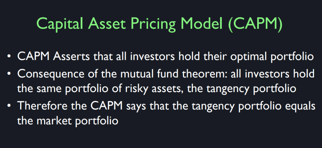
The capital asset pricing model. It’s a model of the optimal portfolio. It asserts that all investors will hold the optimal portfolio. So anyway, I showed you last time a scatter diagram which had on the horizontal axis, the return on the stock market and on the vertical axis, the return on Apple Computer. And there was a scatter of points, one for each year, the return on the market and the return on Apple for that year. And I have fitted a line to that scatter points. The slope of the line is called beta. The idea here is that individuals should diversify. They should hold all the many different eggs in their basket. But diversification is difficult for individual investors. Partly because if you’re a small investor, you’d have to buy fractional shares of each company and you know, the stockbrokers prefer that you do what’s called round lots of 100 shares.
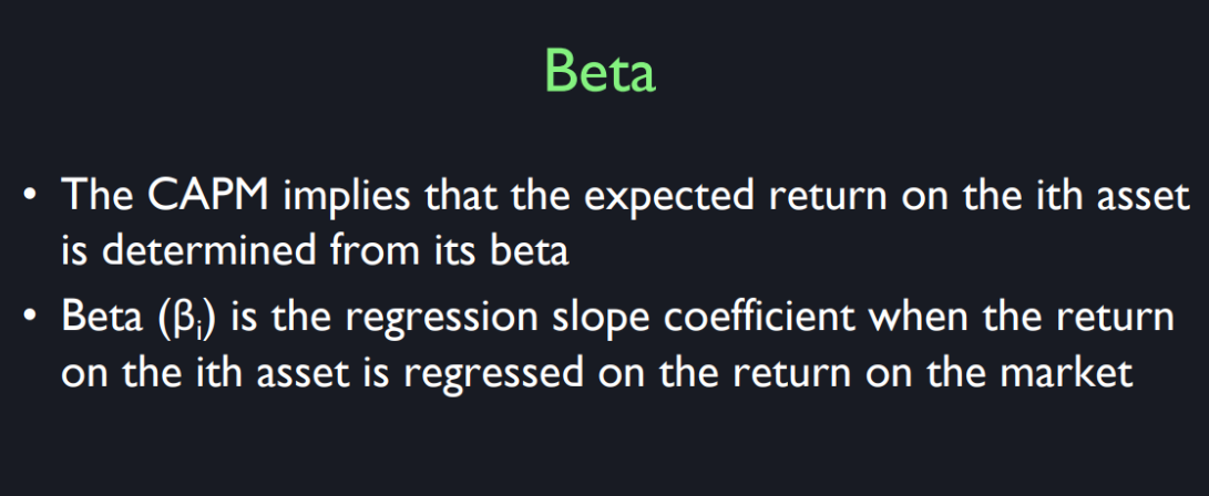
So, you just can’t do it, you’re too small to diversify. So you need some company to help you diversify your portfolio. So, the idea has been going back many decades, that people need investment funds to manage their portfolio for them and the investment funds can diversify optimally for them.
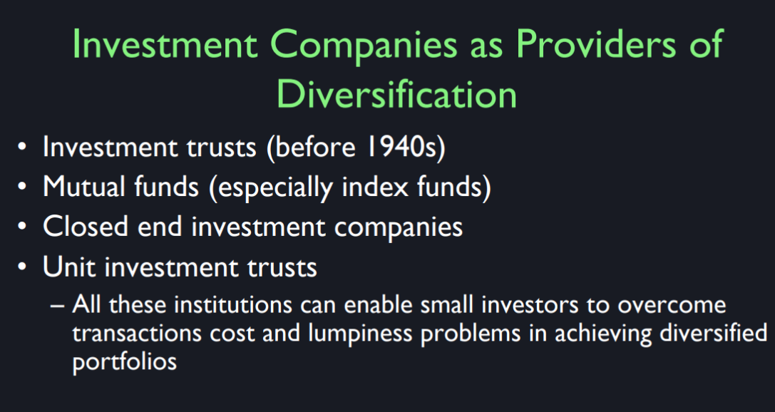
So before the 1940s, we had what were called investment trusts. Later they became a different form called the mutual fund. The first mutual fund is Massachusetts investment trust, MIT, not the institute, in the 1920s but they didn’t really take off until after the 1940s. So a mutual fund or management company, invests in your behalf in assets and it’s mutual in that, it doesn’t skim off profits to a class of stockholders, it’s divided up equally among all the people who invest in the mutual fund. But the mutual fund puts together assets, hopefully, in a diversified manner. So, I know the question of whether we’re really talking about complete diversification or not. Often when we talk about the Capital Asset Pricing Model, or I should say usually, it is assumed that we’re diversifying across all stocks. And maybe all stocks and all bonds. But in fact, if you wanted to be completely diversified, you’d want to include other assets like real estate or commodities like oil, as well. I put this up because I- I had to take a exam to get licensed as a stockbroker at one point in my career till I had a company and it turned out I had to be licensed so I took the exam to become a stockbroker. I never was a stock broker in my life. And the exam study materials is a series seven exam that some of you might end up taking if you go into finance. They talked about classifying all the different investments that someone might make in terms of risk.
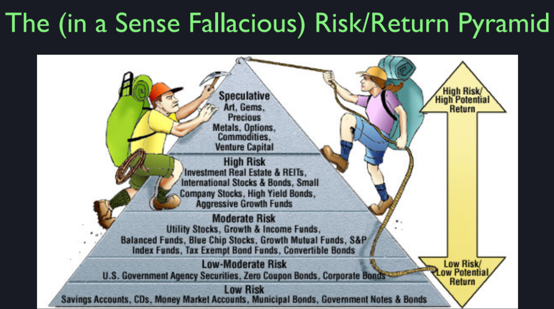
So, there is low risk, moderate risk, moderate risk, high risk and speculative. Now they have a range of mountain climbers climbing to the top. Now they didn’t say what- I had to memorize this for the exam. Something didn’t- bothered me about it though, they didn’t say what you do with this picture of a pyramid. So, it sounds like looking at the picture, like we are supposed to be climbing up to the most speculative investments. I don’t know. But what I thought is, there’s nothing wrong with this diagram, but somehow it’s misleading. What, what CAPM says, doesn’t matter what your risk is, you want to hold all of these. It will average out to be the best for you. So speculative; art, gems, precious metals, options, commodities venture, capital. I want all of them. Okay. Do you want these too? Yes, I want all of them. It’s very simple. It’s not like going to a candy store, you probably just buy one piece of candy. You walk into the candy store and say, “Give me one of everything.” That’s what you should do. Now, if you look historically at different asset classes, you find historically they have paid different amounts out on average through time.
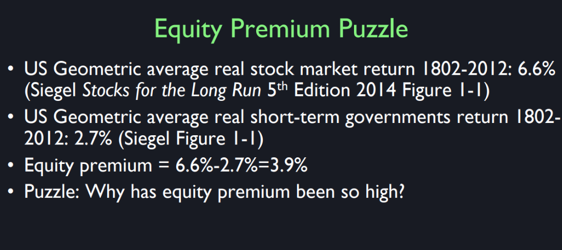
Jeremy Siegel was an old friend of mine at the Wharton School, has just come out with the fifth edition of his book ‘Stocks for the long run’. And he calculates the average return on the stock market in the United States from 1802 to 2012. That’s 210 years of data. It’s a lot of data. And he finds that correcting for inflation. The real inflation corrected return on average for those 200 years was 6.6 % a year. On the other hand, the U.S., the geometric average real short term government return was only 2.7%. So that the equity premium- equity means stocks. The premium of stocks over short term saving vehicles on average for 200 years, was 3.9%. So then, he poses it as a puzzle at the beginning of his book. How can that be? That’s- 200 years is a long time. I’m thinking, everyone this year first thought, should invest in the stock market. Why does anyone invest in short term governments? So this is called the equity premium puzzle. How can it be that one investment has done so much better overall for 200 years compared to another? And that’s what we’re going to try to understand with the capital asset pricing model here.
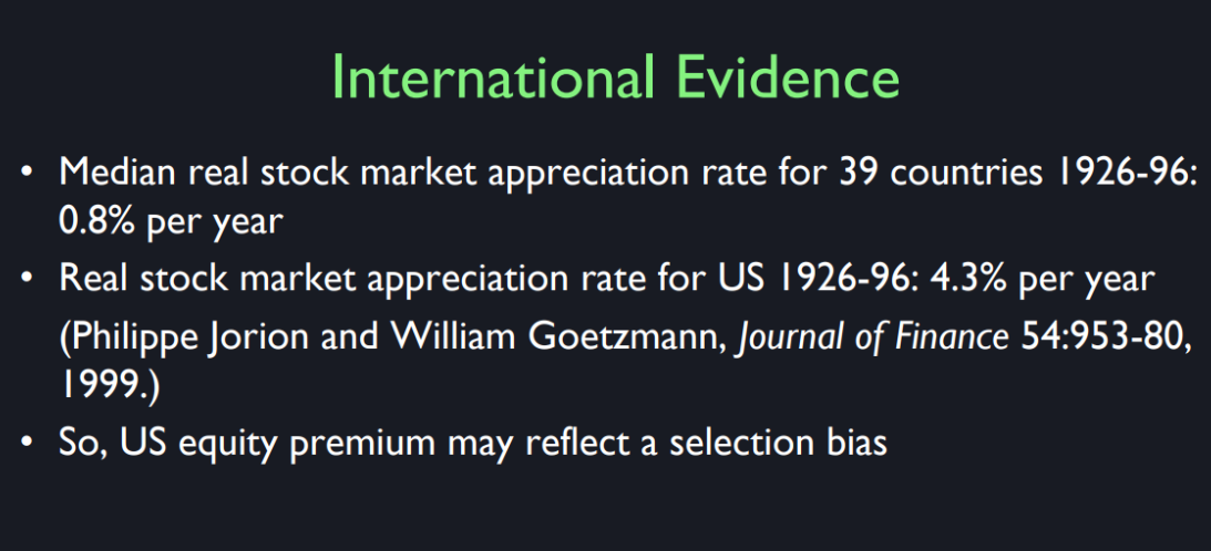
It’s not just for the U.S. but not as dramatically. Will Goetzmann said that to some extent, the U.S. equity premium is a problem of reflex, a selection bias problem. The United States is the most successful capitalist country in the world, you might argue. I mean, someone might try to argue otherwise, but if we’re not we’re pretty close to it. So, you’re looking at the success of stock market investments in the United States is misleading. So you might say, “let’s look at another country, how about Russia?” All right. Well, let’s think, whatever happened in Russia for taking a long from 1802. You know, I kind of remember there was something called the Bolshevik revolution. So basically, it was wiped out. You didn’t get anything. So, they’re not uniformly a good example but at least in the U.S, it seems like now, we may be making a fallacy in assuming that this will is God’s law that stocks outperform other investments but it seems like there have been.
So, do you think that using historic data as a standard deviation or expected return is really helpful in understanding what’s going to happen in the future? Alright. You’re getting at a basic issue is what do we know about the future? And does the past have any indication of the future? Big question. So, let me give you an example; Utilities stocks, that’s electric companies, gas companies. They, they’ve… every month they, they’ve keep the lights on. They’ve been doing this for a long time. So they’re boring stocks and they’d hardly ever have gone bankrupt. So people think those are safe stocks with a low beta or low idiosyncratic variance, and maybe they don’t pay the highest return. Now, and so that would be… that would be supported by data for the last 50 years that they’ve been boring investment. So it almost seems reasonable doesn’t it? That they’re going to continue-what’s exciting about them? You know? But on the other hand, if you look at the history of- I’m just bringing up utilities, they weren’t always boring. Particularly the 1920s, when the world was becoming electrified and electricity was new and these lights were exciting. You’ve switched- in fact that this is an old room, I think you can still see the gaslights. I don’t see them, they remove them. This was obviously lit by gas when it was built, not by electricity. Once the- the electricity is so much brighter and impressive so people were excited about it. So in 1929, that sector that grew the most and crashed was the utilities sector. So, that means you can’t necessarily trust past behavior of stock prices as an indicator of the future. I think that it’s kind of halfway, you can sort of trust it if you know a reason to think otherwise, then you wouldn’t. When you get to other things like Facebook or Google, or whatever, or alphabet, what do you think about their future return? Is that predicted by their past return? Now, who knows? It’s changing, everything is changing too fast.
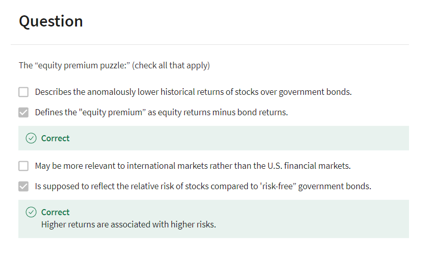
Lumpiness Problem in Achieving a Diversified Portfolio
Overview
The “lumpiness problem” refers to the difficulties investors face in achieving a diversified portfolio due to the indivisible and substantial nature of investments in certain assets. This problem is especially pronounced for individual or small investors who may not have sufficient capital to buy a wide range of assets in the necessary proportions for effective diversification.
Key Issues
Indivisibility of Assets:
- Certain investments, such as real estate or large stock holdings, cannot be easily divided into smaller, affordable units. For example, buying a whole rental property requires a significant lump sum of capital.
High Transaction Costs:
- Small investors often face higher transaction costs relative to their investment size. Buying small quantities of many different stocks can result in disproportionately high brokerage fees and other costs.
Minimum Investment Requirements:
- Many investment opportunities have minimum investment thresholds, which can be prohibitive for small investors. For example, some mutual funds or hedge funds require a minimum initial investment that is beyond the reach of many individual investors.
Round Lots in Stock Trading:
- Stockbrokers typically prefer to deal in round lots (usually 100 shares) rather than odd lots (fewer than 100 shares), which can limit the ability of small investors to diversify their stock holdings efficiently.
Consequences of Lumpiness
Increased Risk:
- Because small investors can’t afford to buy fractional shares of many different assets, they end up with a less diversified portfolio, which increases their exposure to idiosyncratic risk (risk specific to individual investments).
Suboptimal Portfolio Composition:
- Investors might be forced to over-allocate to a few assets they can afford, rather than spreading their investment across a broad range of asset classes, leading to suboptimal returns relative to the risk taken.
Reduced Access to High-Quality Investments:
- Some high-quality investment opportunities, particularly in private equity, hedge funds, and certain real estate projects, are inaccessible to small investors due to their high entry barriers.
Solutions to Lumpiness
Mutual Funds:
- Mutual funds pool resources from many investors to buy a diversified portfolio of stocks, bonds, or other assets, enabling small investors to achieve diversification that would be difficult on their own.
Exchange-Traded Funds (ETFs):
- ETFs allow investors to buy shares in a diversified portfolio of assets. They trade on exchanges like stocks, providing liquidity and ease of access with lower minimum investment requirements.
Robo-Advisors:
- Robo-advisors use algorithms to create and manage diversified portfolios for investors. They often require lower minimum investments and charge lower fees compared to traditional financial advisors.
Fractional Shares:
- Some brokerage firms now offer the ability to buy fractional shares of stocks, allowing investors to invest small amounts in a wide range of companies.
Real Estate Investment Trusts (REITs):
- REITs allow investors to buy shares in a diversified portfolio of real estate properties, providing access to the real estate market without the need to purchase properties directly.
Investment Clubs:
- Individuals can pool their money in investment clubs to collectively invest in diversified portfolios, benefiting from shared knowledge and resources.
Conclusion
The lumpiness problem presents significant challenges for small investors in achieving a diversified portfolio. However, various financial instruments and innovations, such as mutual funds, ETFs, robo-advisors, and fractional shares, offer effective solutions to help overcome these barriers, enabling more individuals to benefit from the principles of diversification.
实现多元化投资组合中的“块状性问题”
概述
“块状性问题”是指投资者在实现多元化投资组合时,由于某些资产不可分割且金额较大的性质而面临的困难。对于个人或小投资者来说,这个问题尤为突出,因为他们可能没有足够的资本购买多种资产,从而难以实现有效的多元化。
主要问题
资产的不可分割性:
- 某些投资(如房地产或大额股票持有)无法轻易分割成小而可负担的单位。例如,购买一整套出租物业需要大量的一次性资金。
高交易成本:
- 小投资者相对于其投资规模往往面临较高的交易成本。购买许多不同股票的小额份额可能导致相对较高的经纪费用和其他成本。
最低投资要求:
- 许多投资机会有最低投资门槛,对小投资者来说可能过于昂贵。例如,一些共同基金或对冲基金要求的最低初始投资额超出了许多个人投资者的承受范围。
股票交易中的整手交易:
- 股票经纪通常更喜欢以整手交易(通常为100股)而不是零散交易(少于100股),这限制了小投资者有效多元化其股票持有的能力。
块状性问题的后果
风险增加:
- 由于小投资者无法负担购买许多不同资产的部分份额,他们最终会拥有一个多元化程度较低的投资组合,从而增加了他们对个别投资特有风险的暴露。
投资组合组成次优:
- 投资者可能不得不在他们能够负担的少数资产上过度配置,而不是将投资分散在各种资产类别上,从而导致相对于所承担的风险而言收益次优。
难以接触高质量投资:
- 由于高门槛的限制,小投资者难以进入某些高质量的投资机会,特别是私募股权、对冲基金和某些房地产项目。
解决块状性问题的方法
共同基金:
- 共同基金汇集众多投资者的资金来购买多元化的股票、债券或其他资产投资组合,使小投资者能够实现他们单独难以实现的多元化。
交易所交易基金(ETF):
- ETF允许投资者购买多元化资产投资组合的份额。它们像股票一样在交易所交易,提供流动性和易获取性,并且最低投资要求较低。
机器人顾问:
- 机器人顾问使用算法为投资者创建和管理多元化投资组合。它们通常要求的最低投资额较低,费用也比传统的金融顾问低。
股票零碎份额:
- 一些经纪公司现在提供购买股票零碎份额的服务,使投资者可以用小额资金投资于许多公司。
房地产投资信托基金(REITs):
- REITs允许投资者购买多元化的房地产投资组合的份额,从而无需直接购买房地产即可进入房地产市场。
投资俱乐部:
- 个人可以通过投资俱乐部将资金汇集在一起,共同投资于多元化投资组合,从而受益于集体的知识和资源。
结论
块状性问题在实现多元化投资组合时为小投资者带来了重大挑战。然而,通过共同基金、ETF、机器人顾问和股票零碎份额等各种金融工具和创新方法,可以有效解决这些障碍,使更多个人能够从多元化原则中受益。
Summary and Key Points of the Lecture
Capital Asset Pricing Model (CAPM)
Overview:
- The CAPM is a model that describes the relationship between systematic risk and expected return for assets, particularly stocks.
- It is used to determine a theoretically appropriate required rate of return of an asset, to make decisions about adding assets to a well-diversified portfolio.
Optimal Portfolio:
- According to the CAPM, all investors will hold the optimal portfolio, which is a diversified mix of all available assets in the market.
- Diversification is crucial as it spreads risk across many assets.
Scatter Diagram and Beta
Scatter Diagram:
- A graphical representation with the return on the market on the horizontal axis and the return on a specific stock (e.g., Apple) on the vertical axis.
- Each point represents the return for a specific year.
Beta:
- The slope of the line fitted to the scatter points.
- Beta measures the volatility of a stock relative to the market. A beta greater than 1 indicates the stock is more volatile than the market.
Diversification and Investment Funds
Need for Diversification:
- Individual investors often struggle to diversify due to the need for significant capital to buy fractional shares.
- Investment funds (mutual funds, etc.) help by pooling resources and diversifying on behalf of investors.
History of Investment Funds:
- Investment trusts were the precursor to mutual funds.
- The first mutual fund was the Massachusetts Investment Trust in the 1920s, but mutual funds became more popular post-1940s.
Mutual Funds and Asset Classes
Function of Mutual Funds:
- Mutual funds pool money from many investors to invest in a diversified portfolio of assets.
- Profits are distributed equally among investors.
Complete Diversification:
- True diversification should include not only stocks and bonds but also other assets like real estate and commodities.
Risk Classification
- Risk Pyramid:
- Investment options can be classified into different risk levels: low, moderate, high, and speculative.
- CAPM suggests holding a diversified portfolio that includes all levels of risk to achieve the best average outcome.
Historical Returns and Equity Premium
Historical Returns:
- Jeremy Siegel’s study shows the real, inflation-adjusted return on U.S. stocks was 6.6% annually from 1802 to 2012.
- The real return on short-term government securities was 2.7%, creating an equity premium of 3.9%.
Equity Premium Puzzle:
- The puzzle lies in why the average return on stocks is significantly higher than that on risk-free assets over a long period.
- This raises questions about why anyone would choose to invest in lower-return government securities.
Historical Data and Future Predictions
Utility Stocks Example:
- Historically, utility stocks are considered safe with low beta and low returns.
- However, during the 1920s, utilities were highly volatile due to the electrification boom.
Predicting Future Returns:
- Past performance is not always a reliable indicator of future returns.
- Especially for rapidly changing sectors like technology, historical data may not accurately predict future performance.
Conclusion
- Diversification Strategy:
- Investors should aim to diversify across a wide range of assets to mitigate risk and achieve better returns.
- Holding a diversified portfolio is recommended over trying to predict the performance of individual assets based on historical returns.
资本资产定价模型(Capital Asset Pricing Model,简称CAPM)是金融学中的一个基本模型,用于确定资产的预期收益率,基于该资产相对于市场的风险。该模型是由威廉·夏普(William Sharpe)、约翰·林特纳(John Lintner)和简·莫辛(Jan Mossin)于20世纪60年代独立开发的。
CAPM的基本公式
CAPM的基本公式为:
[ E ( R i ) = R f + β i ⋅ ( E ( R m ) − R f ) E(R_i) = R_f + \beta_i \cdot (E(R_m) - R_f) E(Ri)=Rf+βi⋅(E(Rm)−Rf) ]
其中:
- ( E ( R i ) E(R_i) E(Ri)) 是资产 ( i ) 的预期收益率。
- ( R f R_f Rf ) 是无风险利率,即在没有任何风险的情况下,投资者可以获得的收益率,通常用政府债券的利率来表示。
- ( E ( R m ) E(R_m) E(Rm)) 是市场组合的预期收益率。
- ( β i \beta_i βi) 是资产 ( i ) 相对于市场的贝塔系数,表示资产 ( i ) 对市场波动的敏感度。
公式解释
无风险利率(( R f R_f Rf )):
- 无风险利率是投资者在零风险下可以获得的收益率。它是所有投资的基础收益率,不受市场波动的影响。
市场风险溢价(( E ( R m ) − R f E(R_m) - R_f E(Rm)−Rf )):
- 市场风险溢价是市场组合的预期收益率减去无风险利率,代表投资者承担市场风险所期望获得的额外收益。
贝塔系数(($ \beta_i$ )):
- 贝塔系数衡量的是特定资产相对于整个市场的波动性。如果 ( β \beta β ) = 1,则资产的波动性与市场相同;如果 ( β \beta β ) > 1,则资产比市场波动性更大;如果 ( β \beta β ) < 1,则资产波动性小于市场。
- 计算贝塔系数的方法是通过回归分析,比较资产收益率与市场收益率的关系,公式为:
[ β i = Cov ( R i , R m ) Var ( R m ) \beta_i = \frac{\text{Cov}(R_i, R_m)}{\text{Var}(R_m)} βi=Var(Rm)Cov(Ri,Rm) ]
其中,( Cov ( R i , R m ) \text{Cov}(R_i, R_m) Cov(Ri,Rm) ) 是资产 ( i ) 的收益率与市场收益率之间的协方差,( Var ( R m ) \text{Var}(R_m) Var(Rm) ) 是市场收益率的方差。
CAPM的假设
CAPM建立在几个关键假设之上:
市场有效性:
- 市场是完全有效的,所有投资者都拥有完全且对称的信息,资产价格完全反映所有已知信息。
投资者行为:
- 所有投资者都是理性的,并且希望最大化他们的投资组合预期收益,基于均值-方差优化。
单期模型:
- 投资者只关注一个投资周期的收益和风险。
无限可分资产:
- 投资者可以无限分割他们的投资组合,以便实现完美多样化。
无摩擦市场:
- 没有交易成本、税收或其他市场摩擦。
CAPM的应用与局限性
应用:
资产定价:
- CAPM广泛用于估算股票和其他证券的预期收益率,从而帮助投资者确定是否进行投资。
资本成本估算:
- 公司常用CAPM来估算其股本的资本成本,这是在评估新的投资项目时的重要参数。
局限性:
假设的现实性:
- CAPM的一些假设(如市场完全有效、投资者理性等)在实际中难以完全满足。
贝塔稳定性:
- 贝塔系数可能随时间变化,导致模型在预测未来收益时可能不准确。
市场组合定义:
- 实际中很难找到一个真正代表市场组合的投资组合。
尽管有这些局限性,CAPM仍然是金融理论中一个重要且广泛应用的模型,提供了一个分析资产风险和预期收益之间关系的框架。
The Capital Asset Pricing Model (CAPM) is a foundational model in finance that describes the relationship between the expected return of an asset and its risk relative to the overall market. Developed by William Sharpe, John Lintner, and Jan Mossin in the 1960s, CAPM provides a framework for understanding how risk and return are connected in a diversified portfolio.
Basic Formula
The basic formula for CAPM is:
[ E ( R i ) = R f + β i ⋅ ( E ( R m ) − R f ) E(R_i) = R_f + \beta_i \cdot (E(R_m) - R_f) E(Ri)=Rf+βi⋅(E(Rm)−Rf) ]
Where:
- ( E ( R i ) E(R_i) E(Ri) ) is the expected return on asset ( i ).
- ( R f R_f Rf ) is the risk-free rate, representing the return on a risk-free investment, typically government bonds.
- ( E ( R m ) E(R_m) E(Rm)) is the expected return on the market portfolio.
- ( β i \beta_i βi) is the beta coefficient of asset ( i ), indicating its sensitivity to market movements.
Explanation of the Components
Risk-Free Rate (( R f R_f Rf)):
- This is the return on an investment with zero risk, serving as the baseline return.
Market Risk Premium (( E ( R m ) − R f E(R_m) - R_f E(Rm)−Rf )):
- The additional return expected from investing in the market portfolio over the risk-free rate, compensating for the extra risk.
Beta Coefficient (( β i \beta_i βi)):
- Measures an asset’s volatility relative to the market.
- A beta of 1 means the asset’s price moves with the market.
- A beta greater than 1 indicates higher volatility than the market.
- A beta less than 1 indicates lower volatility.
Calculation of Beta
Beta is calculated using regression analysis, comparing the returns of the asset to the returns of the market:
[ β i = Cov ( R i , R m ) Var ( R m ) \beta_i = \frac{\text{Cov}(R_i, R_m)}{\text{Var}(R_m)} βi=Var(Rm)Cov(Ri,Rm) ]
Where ( Cov ( R i , R m ) \text{Cov}(R_i, R_m) Cov(Ri,Rm) ) is the covariance between the asset return and market return, and ( Var ( R m ) \text{Var}(R_m) Var(Rm)) is the variance of the market return.
Assumptions of CAPM
CAPM is based on several key assumptions:
Market Efficiency:
- Markets are fully efficient, and all investors have access to the same information.
Investor Behavior:
- Investors are rational and aim to maximize the expected return for a given level of risk, based on mean-variance optimization.
Single Period Model:
- The model considers only a single investment period.
Divisibility of Assets:
- Investors can divide their portfolios infinitely to achieve optimal diversification.
No Transaction Costs:
- There are no taxes, transaction costs, or other market frictions.
Applications and Limitations
Applications:
Asset Pricing:
- CAPM is used to estimate the expected return on stocks and other securities, helping investors decide whether to invest.
Cost of Capital:
- Companies use CAPM to estimate the cost of equity capital, which is crucial for evaluating new investment projects.
Limitations:
Realism of Assumptions:
- Some assumptions, such as market efficiency and investor rationality, may not hold true in reality.
Stability of Beta:
- Beta coefficients can change over time, making future predictions uncertain.
Market Portfolio Definition:
- Identifying a true market portfolio that includes all investable assets is practically challenging.
Despite its limitations, CAPM remains a critical tool in finance, offering a systematic approach to understanding the trade-off between risk and return in investment portfolios.
Chalk Talk: Beta
All right, let’s give an example
of a scatter diagram. And I’m going to pick an example
that compares the return on the stock market, or the overall
market of all investable assets, with the return on an individual stock,
let’s say Apple Computer. Which I just picked because it’s
the biggest company in America. So let me just draw on the horizontal axis the Return on the Market. That’s everything that
you could invest in. We’ll just imagine all
stocks put together. And then on this axis we’re going
to put the return of Apple. And each point represents one year. So let’s pick a year when the stock
market went up, let’s say, the market went up 10%. And what did Apple do in the same year? Let’s say it did 15%. So I make a point here, a point above 10% and at 15% here. In some years the market goes down. Let’s not forget that. So here, I’ll say there was another
year when the market did minus 5%. What did Apple do in that year? Well, let’s say Apple did minus 10%. So, I get a point down here, you see this? This is -10, and this is -5. So I have a point down here. And than I can fill in many year, and each year is a point, and
this is a scatter of points. I’ve got a lot of years showing. And now, when you see this, and
some of them are negative or close to zero, when you see this
scatter of points, you can say well I’m starting to see a relationship here that
there is an upward sloping relation. There’s a positive relation
between Apple and the market.
I can draw a line that’s a best fitting
line through the scatter of points, so that it kind of gets as close as
it can to the scatter of points. That’s called a regression line. And the slope of the line
is called it’s beta. If it has a slope of 1 that means the
stock is reacting 1 for 1 with the market. But in the case of Apple,
the beta is about 1.5. It’s greater than one. The typical stock will just go 1 for
1 with the market. But this is a high beta stock. So it’s reacting more
strongly to the market. >> I see. So then the 1.5 you can see as if
the return of the market goes up, the S&P 500 goes up 10%, then you should have 15% for Apple, which
gives you the beta of 1.5 on average. >> Right, but it won’t be exactly. It doesn’t fall exactly in line.
But they differ from the line, and
that’s called idiosyncratic risk. It’s not related to the market,
it’s Apple risk. So the market could do great in one year. And Steve Jobs could
get sick in that year. It’s just something. So Apple didn’t do well. That’s idiosyncratic. The theory of the capitalized
pricing model is that investors care more about beta than they
do about idiosyncratic risk. because all these companies idiosyncratic
risks will average out and wont matter. What matters is the systematic risk. The risk that correlates with the market. Those things do not average out not matter
how many stocks you put in your portfolio.
And so,
is there any particular reason why some company x would have a high beta versus
another company having a lower beta? >> Well, I think one reason,
there may be many reasons, it’s not just that this
theory doesn’t tell you why. I’m just adding some thoughts on that. One reason why Apple Computer
might be a high beta star, is that it invests in
projects that are iffy, that nobody’s done before. And their success depends on
the state of the economy. So, if they launch a new iPhone
at a time of a severe recession, they’re not going to do well. And the other thing that can make for a high beta stock is that
the company borrows a lot of money. And then they’re playing on the edge,
because they have to make a lot of money or they’ll go bankrupt
cause they borrowed so much. Apple is not in that category,
Apple has not borrowed a lot of money. It has, in fact, a lot of savings. That’s something that
brings its beta down. But Apple is such a lively company, and so connected with what happens
that their beta is still 1.5. >> I see. And so then a counterexample to this might
be if there’s a very low beta stock, so that would kind of look like either
a lower slope or even a negative slope. >> Right, right.
Okay.
So for example, gold might in
many cases be a negative beta stock. Why is that? Because when the stock market crashes
people panic and they get upset, and they want to hold something very safe. At least gold it’s always safe
in one sense, it stays gold. No matter what happens. It’s also something that you can run with. If you think that you’re
going to be a refugee, I want something I can stash in my
purse and just get out of here. Gold has that aspect. So it’s some psychological effect,
that at least in some time periods, it looks like negative beta asset. And then, that would look like this. You have a a scatter diagram
that looks like that. It’s backwards. And you fit a line and it has a negative
slope, you’re going down rather than up. >> Okay, so that means that when the
market is doing well, when the economy’s doing well, gold might not necessarily
be a great option in terms of returns. But then when we have a recession, that’s
when you see returns highest for gold. >> Yeah, and
when constructing a portfolio it matters. Negative beta stocks help
you in a different way. Maybe their return isn’t so
good on average, but they help offset market shocks. So, you’d like to have other things equal, you’d like to have negative
beta stocks in your portfolio. As long as their return isn’t so bad as
to offset the advantage of their beta.
The professor’s lecture explains the relationship between an individual stock’s return and the overall market return using a scatter diagram, focusing on the concept of beta in the Capital Asset Pricing Model (CAPM). Here’s a summary of the key points:
Scatter Diagram and Beta
Scatter Diagram:
- Horizontal axis: Return on the market (overall investable assets).
- Vertical axis: Return on an individual stock (e.g., Apple).
- Each point represents the returns of the market and Apple for a given year.
Plotting Points:
- Points are plotted for each year, showing the relationship between market returns and Apple’s returns.
- Example: If the market goes up by 10% and Apple goes up by 15%, a point is placed at (10, 15). Conversely, if the market goes down by 5% and Apple by 10%, a point is at (-5, -10).
Regression Line:
- A best-fitting line (regression line) is drawn through the scatter of points.
- The slope of this line represents beta.
Beta Coefficient
Definition:
- Beta measures the stock’s sensitivity to market movements.
- A beta of 1 means the stock moves with the market.
- A beta greater than 1 indicates higher sensitivity (e.g., Apple’s beta is about 1.5, meaning it reacts more strongly to market changes).
Interpretation:
- Beta of 1.5: If the market goes up by 10%, Apple is expected to go up by 15%.
- Stocks with higher beta are considered more volatile and riskier.
Idiosyncratic vs. Systematic Risk
Idiosyncratic Risk:
- The risk specific to an individual company (e.g., Apple’s performance may be affected by unique events like the health of its CEO).
- This risk is not related to the market and can be diversified away.
Systematic Risk:
- The risk that affects the entire market.
- Investors care more about beta (systematic risk) since it cannot be diversified away.
Factors Influencing Beta
Nature of Projects:
- Companies investing in innovative or uncertain projects tend to have higher beta.
- For example, Apple invests in new technology, making its success more dependent on the economy’s state.
Leverage:
- Companies with high debt levels may have higher beta due to increased financial risk.
- Apple, however, has significant savings, which usually lowers beta, but its innovative nature keeps its beta high.
Low and Negative Beta Stocks
Low Beta Stocks:
- Stocks with low beta (less than 1) are less volatile than the market.
- Example: Utilities might have low beta because they are stable and less influenced by market fluctuations.
Negative Beta Stocks:
- These stocks move inversely to the market.
- Example: Gold often has a negative beta because it’s seen as a safe asset during market downturns.
- Adding negative beta assets to a portfolio can help offset market risks.
Portfolio Construction
- Diversification:
- Combining different assets, including those with negative beta, can reduce overall portfolio risk.
- The aim is to balance returns with market risks to achieve a stable and diversified portfolio.
In summary, the professor used a scatter diagram to illustrate the relationship between an individual stock’s return and market return, explaining the significance of beta in assessing systematic risk and the importance of diversification in portfolio construction.
Chalk Talk: CAPM and Diversification
Now, we’re talking about the security market line, the basic, the most impressive conclusion of the capital asset pricing model in finance. It is a relationship between the expected return on an asset and its beta. So, what the equation says is that the expected return on the i asset is equal to the risk free rate expected. Actually, it’s the same as the expected because it’s known with certainty plus the beta of the i asset times the return, expected return on the market minus the risk free rate. So, that is the most famous equation.
What it says is that this is a consequence of two things. The theory of forming an optimal portfolio, which we have already discussed, also, the assumption that everybody does it. Okay, now, that second assumption has always bothered me. But, let’s go with it for now. We’re talking about a world in which everyone has a smart money manager who looks at variances in covariances and figures out. Then in that world, it should be that this equation holds, some assets have a higher return than other assets. Does that mean that investors were stupid who invested in the other assets? Absolutely not. The higher return is associated with higher beta which means more risk. And, I’ve just, we’ve just derived what the smart investor would do. And, the smart investor would hold all of the stocks. All of the assets, whether, it’s stocks, bonds and real estate, everything gets held and not everything has the same predicted return.
You can predict that some will earn more than others but it’s always because of higher beta. So, let’s think about this. Some assets have a expected return which is less than the riskless rate. Those are negative data assets, like gold. And so, we say, why would anyone be so stupid as to invest in gold when it has a lower return than the riskless rate? And the answer is, it’s not stupid at all. The negative beta is helping reduce the overall variance of their portfolio. Because gold goes up when the stock market goes down, it offsets other risk. And there are other assets like Apple Computer. We can look back and say wow it had a really high return over the last 20 years. Was I a fool not to put all my money in Apple? No, you weren’t a fool. You did exactly the right thing because, you didn’t know the risk, how the risk outcome would come. You may know that it has a high expected return.
But, Apple is, if you trust the beta, it has a high beta, it’s plunging, it’s a risk, it’s a stock that won’t help you in the stock market crash. Right. And offsetting that, it will really help you a lot in a boom. So, this is a description of a world in which everybody is holding the tangency portfolio. We are not enticed by Apple. We’re not scared off by low return assets. But, it all fits a model of looking at beta and adjusting your portfolio so that you have the optimal mix. It’s kind of a complicated theory because it involves this tangency portfolio, it involves thinking about leverage, it involves thinking about how things move together. But, it is really the core idea in modern finance. That doesn’t mean to say that it’s absolutely right. It’s not absolutely right. It’s only a half truth.
The problem is that not everybody is holding the optimal portfolio. We don’t all own the same portfolio of risky assets. The world isn’t quite consistent with this. But, I think it is a very useful exercise to think about an idealized world where this holds. Is it fair to think of a stock that has a negative beta as being like an insurance, playing an insurance kind of role in your portfolio? Absolutely. A negative beta stock moves opposite other risk. So, you may own Apple computer as an element of your portfolio. But you know, it doesn’t have to work out well. Even though ex ante, the Apple computer was run by brilliant people. History shows, that there is risk in that. And so, you want to have it in your portfolio but you want other things in there as well. And, what you really like, are things like an insurance policy against failure of Apple Computer. Now, you can call that an insurance contract. You could also call it a credit default swap, which is you could focus that on a particular company. But, yes. The the concept of insurance is fundamental to the concept of finance. I don’t know why they separate them out. They’re really two different aspects of the same thing.
So, early on we were talking about gold as being an example, I mean a more modern example, is like when you mentioned the credit default swap. That’s like a contract that is designed to pay out when the market is low. So, it’s like customized beta. Insurance is a different industry, it has different historical origins and it’s regulated differently. So, securities in the United States are regulated by the Securities and Exchange Commission. However, insurance is not regulated by the federal government. It’s regulated by the state governments. And so, it’s different people but, they’re doing similar things. So, really here then I can use this concept to think not only use about stocks and bonds but really derivatives or any kind of asset class potential. Or you can think about, yeah, people make finance analogies to life’s decision.
So, we’re going to come up later about options. But, an option is something you pay for the option to choose later. Some people have said that, “committing yourself to marry someone is like exercising an option.” So, people who are hesitant to commit are just people who have the optimal exercise strategy for their marriage option in mind. That’s a joke. But, it’s not entirely joking. The issues that finance covers are issues that are business analogs of fundamental risks in our lives. And so, you can draw further insights from all this. Then also, I didn’t mean to speak so flippantly about marriage. I’ve been married for 40 years. I don’t think fervently about it at all. But, there is some people who make analogies between business and marriage and other things. And the analogies are not entirely off the mark.
Summary of the Lecture
The professor’s lecture focuses on the Security Market Line (SML) and the key principles of the Capital Asset Pricing Model (CAPM). Here are the main points:
Security Market Line and CAPM
Security Market Line (SML):
- The SML represents the relationship between the expected return on an asset and its beta.
- The equation for the SML is:
Expected Return on Asset i = Risk-Free Rate + β i × ( Expected Return on Market − Risk-Free Rate ) \text{Expected Return on Asset i} = \text{Risk-Free Rate} + \beta_i \times (\text{Expected Return on Market} - \text{Risk-Free Rate}) Expected Return on Asset i=Risk-Free Rate+βi×(Expected Return on Market−Risk-Free Rate) - This equation is derived from the theory of forming an optimal portfolio and the assumption that all investors follow this theory.
Implications of the SML:
- Higher beta means higher risk and higher expected return.
- Negative beta assets, like gold, may have expected returns lower than the risk-free rate but are still valuable as they help reduce the overall portfolio risk by offsetting market downturns.
Optimal Portfolio:
- In the idealized world of CAPM, investors hold a tangency portfolio that includes all assets (stocks, bonds, real estate).
- The portfolio is constructed based on beta, not individual expected returns.
- Investors are not considered foolish for holding assets with lower returns if those assets help reduce overall portfolio risk.
Understanding Beta and Risk
High Beta Stocks:
- Example: Apple Computer, with a beta of about 1.5, meaning it is more sensitive to market changes.
- High beta indicates higher risk and higher potential return, but also higher volatility.
Negative Beta Stocks:
- Example: Gold, which typically has a negative beta because it tends to rise when the market falls.
- These stocks act as a form of insurance, reducing portfolio risk during market downturns.
Practical Considerations
Real-World Application:
- Not everyone holds the optimal portfolio as assumed in CAPM.
- Understanding CAPM helps in constructing a diversified portfolio that balances risk and return.
Insurance and Finance:
- Negative beta assets or instruments like credit default swaps act like insurance, providing protection against specific risks.
- The concept of insurance is integral to finance, despite being regulated differently.
Analogies to Life Decisions:
- Financial concepts like options can be analogous to life decisions, such as marriage.
- Understanding finance can provide insights into various aspects of life beyond just investments.
Conclusion
- CAPM and the SML provide a framework for understanding the relationship between risk and return in an idealized market.
- The model emphasizes the importance of diversification and the role of beta in constructing an optimal portfolio.
- While the real world may not perfectly align with the model, the principles of CAPM remain fundamental to modern finance.
The phrase “everybody is holding the tangency portfolio” refers to an idealized scenario in the Capital Asset Pricing Model (CAPM) where all investors construct their portfolios in the most efficient way possible given their risk preferences. Here’s a breakdown of what this means:
Tangency Portfolio:
- The tangency portfolio is the optimal mix of risky assets that, when combined with a risk-free asset, provides the highest possible return for a given level of risk.
- It is the point on the efficient frontier (a curve representing the best possible risk-return combinations) that is tangent to the capital market line (CML), which represents the risk-return trade-off at different levels of leverage.
Capital Market Line (CML):
- The CML shows the relationship between risk (as measured by the standard deviation of portfolio returns) and expected return for efficient portfolios that combine the risk-free asset with the tangency portfolio.
- The slope of the CML is the Sharpe ratio of the tangency portfolio.
Holding the Tangency Portfolio:
- In the CAPM world, it is assumed that all investors, regardless of their individual risk tolerance, will hold the tangency portfolio of risky assets. The difference in their portfolios comes from the proportion they invest in the tangency portfolio versus the risk-free asset.
- Investors with high risk tolerance will leverage the tangency portfolio (borrowing money to invest more in it), while more risk-averse investors will combine the tangency portfolio with a significant portion of the risk-free asset.
Key Implications
- Diversification: Holding the tangency portfolio implies that investors are fully diversified across all risky assets in the most efficient manner possible.
- Market Efficiency: The assumption that everyone holds the tangency portfolio implies that markets are efficient and all available information is reflected in asset prices.
- Systematic vs. Idiosyncratic Risk: The tangency portfolio considers only systematic risk (market risk), as idiosyncratic risk (specific to individual assets) is diversified away.
Why It’s Idealized
- Real-World Deviations: In reality, not all investors have the same information, risk tolerance, or investment constraints. As a result, not everyone holds the tangency portfolio.
- Behavioral Factors: Human behavior, such as overconfidence or aversion to loss, can lead to deviations from the optimal portfolio suggested by CAPM.
In summary, “everybody is holding the tangency portfolio” represents an idealized scenario in CAPM where all investors optimally diversify their investments to achieve the best possible risk-return trade-off, aligning their portfolios along the capital market line.
“everybody is holding the tangency portfolio”这句话在资本资产定价模型(CAPM)中指的是一个理想化的情景,即所有投资者都按照他们的风险偏好,构建出最有效的投资组合。具体来说,这意味着:
切点投资组合:
- 切点投资组合是将所有风险资产按照最优比例组合在一起,以达到在给定风险水平下的最高预期收益的投资组合。
- 在有效边界(代表最佳风险-收益组合的曲线)上,这个投资组合与资本市场线(CML,即不同杠杆水平下的风险-收益权衡关系线)相切。
资本市场线(CML):
- 资本市场线显示了组合风险(以收益率的标准差衡量)与预期收益之间的关系,适用于那些将风险资产与无风险资产结合起来的有效投资组合。
- CML的斜率是切点投资组合的夏普比率(Sharpe Ratio)。
持有切点投资组合:
- 在CAPM世界中,假设所有投资者,无论其个人风险承受能力如何,都会持有切点投资组合的风险资产。不同之处在于他们在切点投资组合和无风险资产之间的投资比例。
- 高风险承受能力的投资者会杠杆化切点投资组合(借钱投资更多),而风险厌恶型投资者会在切点投资组合中加入大量无风险资产。
关键含义
- 分散投资:持有切点投资组合意味着投资者在所有风险资产中进行了最有效的分散投资。
- 市场效率:假设每个人都持有切点投资组合意味着市场是有效的,所有可用信息都反映在资产价格中。
- 系统性风险与非系统性风险:切点投资组合仅考虑系统性风险(市场风险),因为非系统性风险(个别资产特有的风险)已经被分散掉了。
为什么是理想化的
- 现实中的偏离:现实中,并非所有投资者都有相同的信息、风险偏好或投资限制。因此,并不是所有人都持有切点投资组合。
- 行为因素:人类行为,如过度自信或损失厌恶,可能导致偏离CAPM建议的最优组合。
总之,“everybody is holding the tangency portfolio”表示在CAPM中一个理想化的情景,即所有投资者都按最优方式分散投资,以实现最佳的风险-收益权衡,使他们的投资组合沿着资本市场线排列。
Short Sales
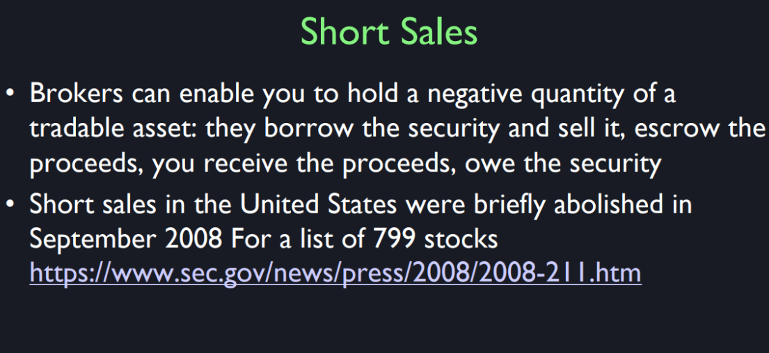
If we were to compute
the optimal portfolio, given the risk and
return of individual stocks, how do we know that you won’t want to
hold negative quantities of some assets? So that’s what’s called a short sale. You can, in most countries of the world,
you can hold negative quantities of a stock just as
well as you can hold positive quantities. If you get one of those online
brokerage service sites, you have to maybe sign up for
a special account to do short sales. But you can say I’d like
to short this stock. So how do you own a negative
quantity of a stock? What it means is you borrow the shares and
you sell them. Now you owe the share to someone else. The stockbroker can help you do that,
and it’s very routine these days. For centuries it’s been very routine. Most investors don’t do it. So you could buy a negative
quantity of a stock. Why would you do that? Well, you would do that disregarding
the cap M that we’re talking about. You might say you would do that if you
think the price is going to go down. If the stock is overpriced,
it doesn’t look good. Instead of not buying it,
I’ll buy a negative quantity of it. Capital asset pricing model assumes that,
yeah, you can buy positive or negative amounts.
Let’s find the optimal portfolio. But then it turns out, however,
that if you really take the idea that everyone would do the same thing,
no stock could ever have an optimal holding of a negative number because there
would be a negative holding for everybody. And everyone would want to short it,
and that can’t add up. So we’re going to allow
short sales in our math, but we’ll assume that they won’t happen,
not on average. >> Here’s why short sales won’t happen. In our model, the optimal portfolio
decision of all investors in equilibrium will be symmetric or
identical. Given that, we can conclude that no
single investor will ever short a stock in equilibrium because then everybody in
our model would be shorting that stock. Which brings up the question, who is
providing the stock for you to short? >> So what I’m really coming up to
is a kind of abstract model, and I’d like to talk about the real world. But the capital asset pricing
model is a little abstract. So what it assumes is that
everybody is rational. It assumes that nobody has any
risks that are inherent to them. They all want to do the same thing except
for maybe a variation of leverage. They all want to do the same thing. And so as a result,
nobody will ever short a stock. Now this is an abstract model, and
I have to apologize a little bit for it, because there are short sales. But it’s a model, and
it’s actually a very important model. By the way, the United States government
has historically allowed short sales, but they were briefly abolished. The US government got so scared that there
would be a 1929-style stock market crash, that it made a temporary
law against short sales. No one was allowed to
short these 799 stocks. So we’re going to develop a theory that
puts no short sale restrictions on it. We’re going to assume that
everyone does careful calculations of the mean and standard
deviation of their portfolio return. And let’s see what that implies. What it does imply is that there
will be a optimal portfolio and we should be on what’s called
an efficient portfolio frontier. I won’t explain this. This is from David Swenson’s book about how he moved Yale
to the optimal portfolio. When he took over management of
Yale’s portfolio, it was originally not well managed, and it was not optimal. So here, this is his account
of the movement of the L portfolio toward the efficient frontier
of between 1990 and the year 2000. So we have scientific management
of portfolios here at Yale. So we’ll come back to
understanding what this is.
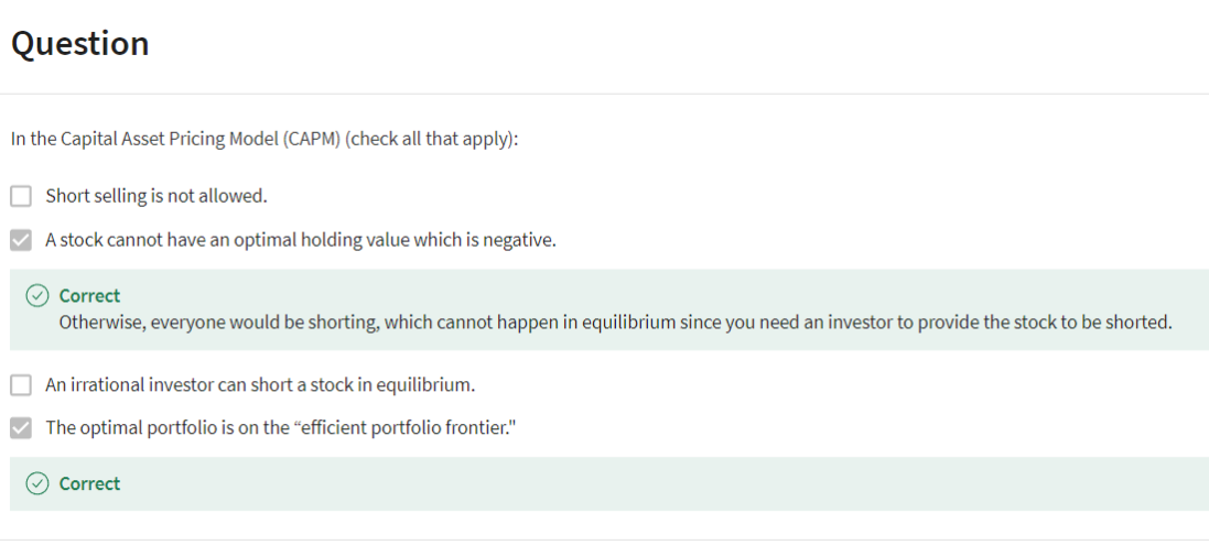
So just a general question about investing. How are sort of unsophisticated,
middle-class people supposed to invest their money now with
the interest rates so low? What is there to do? Like what can you do? >> Well, interest rates are starting
to go up, so maybe wait five years. [LAUGH] Now here is a fundamental
issue about rationality. And most people are not financial wizards, as your question implies. And so what should we do? Should we have the government invest for
them? Somehow there’s something wrong about
that, too, because the governments don’t have a particularly good record
of deciding how to investments either. The United States has been an example of
capitalist institutions going way back. We have had lively stock markets and other kinds of speculative markets. People have lost money and had been
taken advantage of over the years. But on the other hand,
it produces an atmosphere of attention to business that produces a general
culture of sympathy to business. If you invest in businesses,
then you’ll be less likely to vote for a strong man leader who
will corral businesses. So the US has set an example
to the world about. Just letting some of these things happen. So you’ve got this guy, Thomas Edison, with these electric lights,
he might be a nut, who knows. But some people invested in him. And there were other stories
that didn’t work out so well. But on balance, over 100 or 200 years the US system has looked pretty good and it’s become spread. I mean, not just the US’s but
I’m saying having free markets and involving people at large in
some investing decisions, it has worked out well, even though it
doesn’t work out well for everyone.
Hold negative quantities of a stock
“Hold negative quantities of a stock” 的意思是投资者卖空股票。卖空(short selling)是一种投资策略,投资者通过借入股票并立即出售,期望在未来以更低的价格买回这些股票来实现盈利。这样,他们实际上持有负数量的股票。
详细解释
借入股票:
- 投资者从经纪人或另一方借入股票,这些股票并不属于投资者本人。
卖出股票:
- 投资者立即卖出借来的股票,希望价格会下跌。
回购股票:
- 在未来某个时候,投资者以较低的价格买回相同数量的股票,并将其归还给出借方。
实现利润:
- 如果股票价格下跌,投资者以低价买回股票,就能从中赚取差价(卖出时的高价减去买回时的低价)。
例子
假设投资者A认为公司X的股票(当前价格为每股$100)会下跌。A从经纪人那里借入100股公司X的股票,并以$100的价格卖出。这时,A“持有负数量”的股票,即 -100股。如果股票价格如A预期的那样下跌到$80,A以$80的价格买回100股股票,并归还给经纪人。A的利润为:
[$ ($100 - $80) \times 100股 = $2000 $ ]
风险
无限风险:如果股票价格不跌反涨,投资者A将面临潜在的无限损失。例如,如果股票价格涨到$150,A将不得不以每股$150买回股票,这将导致每股$50的损失,总共是$5000的损失。
借贷成本:借入股票的成本和维持保证金账户的费用也需要考虑在内。
为什么卖空
- 看跌策略:投资者认为股票价格会下跌。
- 对冲策略:作为其他投资组合的对冲措施。
总结
“Hold negative quantities of a stock” 意味着投资者卖空股票,通过借入并卖出股票,期望在价格下跌时买回股票以实现盈利。这是一种高风险高回报的投资策略。
“Holding negative quantities of a stock” means that an investor is short selling the stock. Short selling is an investment strategy where the investor borrows shares and sells them, hoping to buy them back later at a lower price to make a profit. Essentially, the investor is betting that the stock’s price will decline.
Detailed Explanation
Borrowing Shares:
- The investor borrows shares of the stock from a broker or another party.
Selling the Shares:
- The investor sells the borrowed shares immediately at the current market price.
Repurchasing the Shares:
- At a future time, the investor buys back the same number of shares, ideally at a lower price.
Returning the Shares:
- The repurchased shares are returned to the lender.
Profit Realization:
- If the stock price has fallen, the investor profits from the difference between the selling price and the lower repurchase price.
Example
Suppose investor A believes that the stock of company X (currently priced at $100 per share) will decrease in value. A borrows 100 shares of company X from a broker and sells them at $100 per share. Now, A “holds negative quantities” of the stock, specifically -100 shares. If the price of the stock drops to $80, A buys back 100 shares at this lower price and returns them to the broker. A’s profit is calculated as follows:
[ $($100 - $80) \times 100 \text{ shares} = $2000$ ]
Risks
Unlimited Risk: If the stock price rises instead of falling, the investor faces potentially unlimited losses. For example, if the price increases to $150 per share, the investor must buy back the shares at this higher price, resulting in a loss of $50 per share, or $5000 total.
Borrowing Costs: There are costs associated with borrowing the shares and maintaining a margin account.
Why Short Sell?
- Bearish Strategy: Investors short sell when they expect the stock price to decline.
- Hedging Strategy: It can be used as a hedge to protect other investments in the portfolio.
Summary
“Holding negative quantities of a stock” means that the investor has sold short. They have borrowed and sold shares, hoping to buy them back at a lower price in the future to realize a profit. This strategy carries high risk and high potential reward.
Calculating the Optimal Portfolio
Yeah, capital as a pricing model is based on rational markets and rational investors, right? What does it mean to be rational? And maybe you could explain what the saying is “The market can stay irrational longer than you can stay solvent”. What does it mean to be rational? I’m married to a psychologist but you can ask my wife. We’re economists. We have a very simple model of people. But what does it mean to be rash- Sometimes I think rational people, they don’t pay attention to financial markets at all. They’re in the important things like making friends. But on the other hand, there is some basic simple notion of human rationality that is I think it’s partly correct. People are partly rational. But they often make mistakes. This is something we’re going to talk about in the semester. Behavioral finance is an important field. And we mostly think of ours- Do you think of yourself as rational? Sometimes. I don’t know if we have agreement on this about who’s- I never thought of myself as particularly rational. I have trouble with self-discipline. Do you ever get lazy? Yeah. Well, that’s part of irrationality. Or do you ever find that you’re just following entertainment? You’re just bored with getting the facts. You want to hear entertainment. [inaudible] So these are human traits. The capital asset pricing model, the heroic assumption that is often taken uncritically is that everybody is investing according to that model. Now, on the face of it, that is absolutely absurd because if you asked the population to describe the capital asset pricing model, it wouldn’t be more than one in a hundred who would know what you’re talking about. To assume that they’re just doing it, it’s pretty extreme. On the other hand, I still like to go through the mathematics and see what would it be if everybody were extremely rational and logical, and how would the markets behave. It’s interesting.
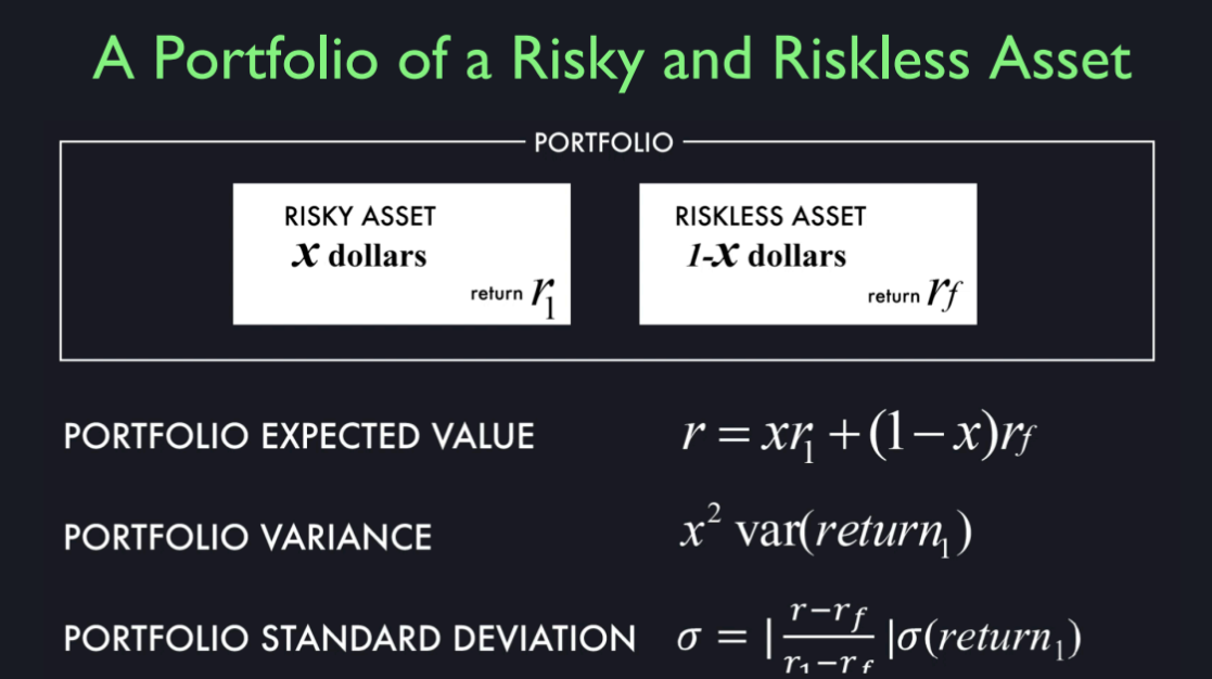
So, let’s just think about one risky asset and one risk-less asset. Suppose I put X dollars into a risky asset one. Now I’m going to invest $1 total. I’m just normalizing it on one dollar. So the money I have left over after I invest X is 1-X, to help with that in the second asset, which is earning a sure but low return of rf. So what is the expected value of the return on my portfolio? Well, I have X dollars in the first asset so it’s going to be X times the expected return on the first asset. The risky asset. And I’ve got 1-X dollars in the risk-less rate. And so, the total expected return is Xr1+1-X* rf.
And so, what is the variance of my return? Or the variance is just equal to X squared times the variance of the return on the first asset. So, if X is one, that means I put it all in the first asset, then it’s just the portfolio variance is the variance of the return on the first asset. What if I shorted? I put minus one. If I shorted, that wouldn’t be- It doesn’t sound like a smart move, generally, on average shorting the stock market and investing in the risk-less asset. But I could do that. I could make X= -1, and then I would have $2 invested in the risk-less asset. My portfolio variance would be the same, but I’d be on the wrong end of it, right? Assuming that I’ve got my numbers right, I would be shorting the high return asset and investing in the low return asset. So, and having the same risk anyway.
You can compute the portfolio of standard deviation which is just the square root of this portfolio variance. So it’s linear. The standard deviation of the portfolio is linear in the expected return on the portfolio. See, the real answer here as, I tried to convey that last time. You want an expected return, I can give it to you on stocks and anything you want, but I’ll do it by exposing you to risk. I can leverage you up. You want a 100 percent expected return next year? Great. I’ll leverage it to the hilt. And then you’ll have that expected return which will probably get wiped out because you’ve taken on to leverage than investment.
Let’s illustrate the idea of how levering up to the hilt can give you any expected portfolio return you want. Let’s say you start with $1 and there are only two investable assets in the world. Let’s look at a risky asset which offers an expected return of 20% and a return standard deviation of 5%. And the other asset is the risk free asset which guarantees a return of 10% with no risk. If you want 100% expected return on your $1 portfolio. First, borrow, AKA “short”, $8 from the risk free market, and now you have $9 to play with. Invest all $9 in the risky asset.
This provides you with an expected return next period of 20%. So your portfolio now has $10.80 on average. Pay back what you owe which is 8*1.1 or $8.80, you’re left with $2 in your portfolio and you have thus doubled your initial investment on average. Remember though, you took on an 8 to 1 leverage ratio to get here. Using the formula the standard deviation of your portfolio return was 9 * 5%, or 45%. If the risky asset realized any return less than -2.2% which is half of one standard deviation away from the mean, you would have to file for bankruptcy.
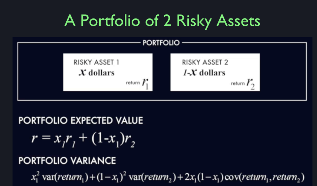
But we’re not going to worry about being wiped out here, we’re just worrying about what your return will be. Now, suppose we move from just one risky asset to two risky assets. Now, I want to put $X1 in risky asset one, and 1-$X1 in risky asset two. What is the portfolio expected return? And I’m not putting anything into the riskless asset. So now I have two risky assets. The expected value of the return on my portfolio is equal to X1 which is the dollars I put in asset 1, times the expected return on an asset one, plus one minus X1 dollars.
Now what is the variance of this portfolio? It turns out this is the formula. The variance of the portfolio is X1 squared times the variance of the return on the first one, plus 1-X1 squared times the variance of the return on the second risky asset, plus 2X1*1-X1 times the covariance of the returns.
Now the covariances matter because if they covariate positively, that makes them interact in a positive way increasing variance. So, positive covariance is bad for your portfolio. It raises the variance of your portfolio. Negative covariance is good. If you can find two risky assets that move opposite each other or tend to move opposite each other, then there covariance is negative and this thing reduces the portfolio variance. What we’re doing with the CAPM is that we’re moving beyond Mr. Crumb’s day. We now have statistics. And so, I’m imagining here that you are managing a portfolio and you have historical data on the returns of the different assets that you can put into the portfolio. So you’ve calculated what the expected return is for the first asset, the average historically for its return. You’ve calculated what the expected return on the asset, second asset is. You’ve taken an average. You’ve also computed the variances of the returns. So you know how variable they are. And you’ve even calculated the covariance of the returns. Now, you might question whether covariances, variances, expected values that I estimated historically will continue to be true in the future. Maybe things are different now. But at least as a first exercise, it sounds like this is something we should understand, doesn’t it? It’s a first guess. We’ll assume that these variances are going to be stable through time. So I want to know, what I should do if I assume they are stable through time? That’s the key idea. And that had not been worked out until Harry Markowitz developed the capital asset pricing model in the early 1950s.
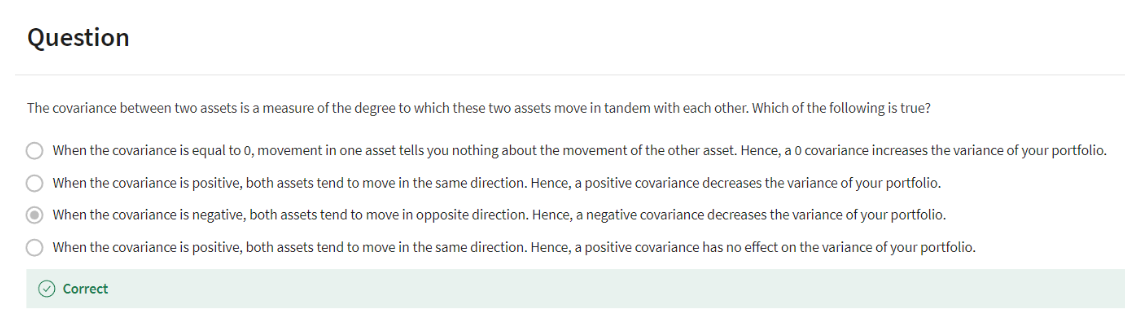
Let’s examine each statement:
“When the covariance is equal to 0, movement in one asset tells you nothing about the movement of the other asset. Hence, a 0 covariance increases the variance of your portfolio.”
- Partially True: The first part is true: a covariance of 0 means the movements of the two assets are independent of each other. However, the second part is false: a 0 covariance neither increases nor decreases the variance of your portfolio. It simply means there is no relationship between the movements of the two assets.
“When the covariance is positive, both assets tend to move in the same direction. Hence, a positive covariance decreases the variance of your portfolio.”
- Partially True: The first part is true: a positive covariance means that both assets tend to move in the same direction. However, the second part is false: a positive covariance increases the variance of your portfolio because the assets’ movements reinforce each other.
“When the covariance is negative, both assets tend to move in opposite direction. Hence, a negative covariance decreases the variance of your portfolio.”
- True: Both parts of this statement are true. A negative covariance means that the assets tend to move in opposite directions, which helps to reduce the overall variance of the portfolio by providing a natural hedge.
“When the covariance is positive, both assets tend to move in the same direction. Hence, a positive covariance has no effect on the variance of your portfolio.”
- Partially True: The first part is true: a positive covariance means both assets tend to move in the same direction. However, the second part is false: a positive covariance does have an effect on the portfolio variance, increasing it.
Correct Statement:
“When the covariance is negative, both assets tend to move in opposite direction. Hence, a negative covariance decreases the variance of your portfolio.”
This is the accurate statement. Negative covariance between two assets means that when one asset’s return goes up, the other asset’s return tends to go down, and vice versa. This negative correlation helps to reduce the overall risk (variance) of the portfolio.
Summary of the Lecture
Rationality in Financial Markets
- Rationality: In economics, rationality involves making decisions based on logic and facts to maximize utility. However, human behavior often deviates due to emotional and psychological factors.
- Behavioral Finance: A field that studies the effects of psychological influences on investors and markets.
Capital Asset Pricing Model (CAPM)
- Assumptions: CAPM assumes that all investors are rational and markets are efficient. This is unrealistic as most people don’t fully understand or follow CAPM in their investments.
- Key Equation: Expected return on an asset = Risk-free rate + (Beta of the asset * (Expected return on the market - Risk-free rate)).
- Beta: Measures an asset’s sensitivity to market movements. A higher beta indicates higher risk and potentially higher returns.
Optimal Portfolio
- Tangency Portfolio: The portfolio that optimally combines risk and return by holding all available assets in proportions that maximize return for a given level of risk.
- Expected Return and Variance: The expected return of a portfolio is a weighted average of the returns of individual assets. Variance (risk) is calculated considering the variances of individual assets and their covariances.
Leverage and Short Selling
- Leverage: Borrowing money to invest more than one’s own capital. This can amplify both gains and losses.
- Short Selling: Selling borrowed stocks with the hope of buying them back at a lower price.
Portfolio Management
- Single vs. Multiple Risky Assets: Managing a portfolio with multiple risky assets involves considering the expected return and variance of each asset as well as their covariances.
- Covariance: Positive covariance increases portfolio risk, while negative covariance reduces it.
Practical Application
- Historical Data: Portfolio management relies on historical data to estimate expected returns, variances, and covariances.
- Challenges: The stability of these estimates over time is uncertain, making it a challenging but essential exercise.
Key Insights
- Realistic Market Behavior: Despite the assumptions of CAPM, real market behavior includes irrational actions by investors.
- Risk and Return Trade-off: Higher expected returns come with higher risk. Diversifying a portfolio can help manage risk through negatively correlated assets.
- Leverage Risks: While leverage can increase potential returns, it also significantly increases risk, potentially leading to insolvency.
This lecture emphasizes the importance of understanding both theoretical models like CAPM and the practical aspects of portfolio management, acknowledging the limitations and behavioral aspects that influence real-world investing.
Efficient Portfolio Frontier
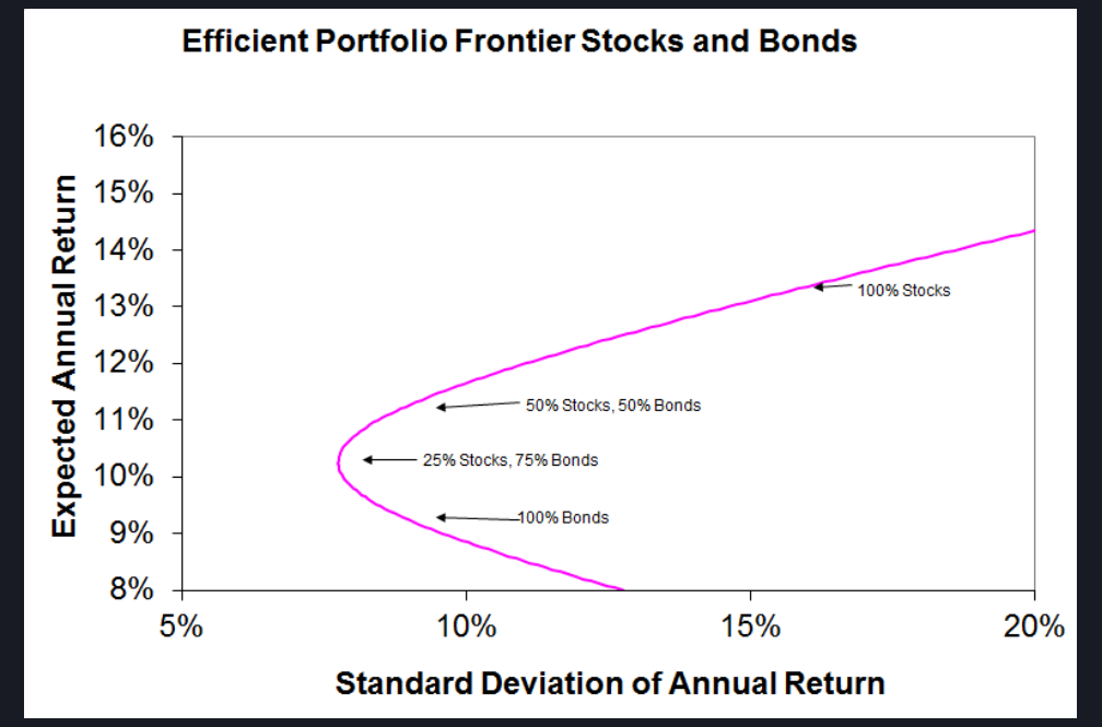
So, what I want to do now is calculate the efficient portfolio of frontier which expresses the standard deviation of the portfolio in terms of r the expected return on the portfolio instead of X-1. So here is an example of the efficient portfolio frontier, I calculated for two investments, U.S. stocks and U.S. bonds using their historical expected returns, standard deviations, and covariances, variances and covariances. So what we have on this axis is the standard deviation of return and we have on this axis the expected annual return. So, and these are the possibilities we calculate with a formula.
Let’s consider a couple of special cases I have shown here. I can put all my assets in the stocks and then I would get an expected return equal to the return on stocks or I can invest entirely in bonds and I would be at this point here on the diagram. Bonds, these are long term bonds, they’re risky because they’re long term.
Here, Professor Shiller mentions bonds are risky because they’re a long term. I wouldn’t fixate too much on the use of the term bonds here. We’re analyzing the efficient portfolio frontier with any two risky assets. In this case he chose the example of stocks and bonds to emphasize that there are two separate types of assets. You could easily replace the word stocks and bonds with Microsoft stock and Tesla stock and the argument still works.
Have historically, had a lower standard deviation of annual return but also a lower expected return. So I could achieve that by putting all of my money in bonds and I can achieve this by putting all of my money in stocks. What if I put half my money in stocks and half in bonds that puts me right here. So what we see is that there’s an infinite number of possibilities. Oh, by the way, I could go more than 100% stocks if you like, I can go out here. So that looks like it’s something like 120% in stocks and -20% in bonds. So to do that I’d have to short the bond market and buy the stock market. I can do that, I can do anything. It’s just those two formulas that I just showed or the single formula for this curve.
So what do you like? If you are investing your money and I showed you this, what would you pick? If Suppose you picked here then another adviser would come up and say, “you idiot, you could have picked up here and then you would have gotten more return”. And note, no difference in risk, shorting the stock market is risky. If it has a negative expected return you don’t want to do that. So what that means is that the hope curve here, below the minimum variance point is dominated, it’s called the dominated. You don’t ever want to be there. Well, what David Swensen says, “you know who is there before he arrived? Yale University was there.” They had some fuddy duddy investment advisors who would say, “you know we’ve advised endowments of portfolios over the years and we find that for institutions like the Yale University they would do well to put their money in sound safe government bonds.” And so, actually it wasn’t David Swensen who first pointed out the foolishness of it. It was starting to come in with the whole capital asset pricing model. I think there was a Ford Foundation study of university endowments in the 60s that pointed out that universities are just stupidly putting their money in bonds. It used to be considered just smart, you know it was almost like religion, you had to do things the right way. In Europe, a lot of… a lot of foundations have put all their money in bonds because that was supposed to be safe. And then in Germany, in the 1920s, there was a hyperinflation in 1923. Every foundation in Germany was completely wiped out by the hyperinflation, they should have thought of this. It wasn’t safe and they were undiversified and they were doing the under-performing under diversified asset.
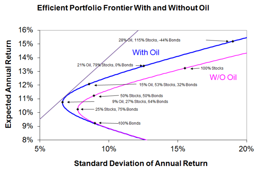
So, but it still takes a while you know you have university corporations or boards tend to be filled with various old fashioned educators. They can’t imagine putting money in the stock market but David Swensen change that. So you don’t ever want to be down here but you want to pick some point up here depending on your risk and it’s a matter of taste where along this frontier you choose to go. So, here now I have the same curve that I showed you before for stocks and bonds and now let’s add a third asset called oil. Okay? I did this with actual variances and covariances when I did this diagram. Forget this diagonal line for the moment, now I have three assets: stock, bonds, and oil. And so what is the minimum varian- minimum standard deviation I can get for any given expected return? And you can see there it gets more complicated now. The minimum variance portfolio… the minimum standard deviation portfolio would be 9% oil, 27% stocks and 64% bonds. Up here, this is 21% oil, 79% stocks, 0% bonds and here is 28% oil, 115% stocks, -44% bonds. All those things are possible and so, now you might say I should take the minimum standard deviation, shouldn’t I? Or is that right? Well, not generally, right, because you’re sacrificing some return for that. You have to pick a point that reflects your tastes. So, now that we’ve added oil, you should not own a portfolio with just stocks and bonds in it, it’s because the new portfolio frontier dominates. In other words, you can get the same return with a lower standard deviation. So putting our oil as a risky asset as you know recently. I’ve did this chart some years ago, so this is not updated but what we’re seeing lately confirms oil is risky. It has… it was up to $150 a barrel or over that in 2008 and now it’s under $30 a barrel, it’s jumping around wildly. So you might say, “I’m going to stay away from oil.” The answer is, “no you shouldn’t, you should have if you want everything in your portfolio.” But maybe you want something like this point. So you’re only 21% exposed to oil, 79 % stock, that sounds like a reasonable point. There are various possibilities here but the point is you don’t want to… you don’t want to just invest in stocks and bonds. Once you add oil there’s more… there’s more opportunity to achieve expected return without risk.
Today’s economy, there’s so much uncertainty and many potential investors I think are fear- fearful of getting involved in the market. Is there a message that you think you would share with potential investors about what’s going on today with fluctuating markets and how to kind of continue to stimulate our economy. Well it’s going to be a mixed message. There is something inherently unsatisfying about investing in the stock market because you are putting yourself on the line for risks in so many different ways. And you can’t possibly assess them all. Risks of financial crisis, risks of, I would say psychologically induced panics and so many people around the world have concluded-- I’m just going to stay out of stocks for example, because it’s just a quagmire. I know that… I know that I can’t figure out these investments and people are trying to sell me on this. I don’t trust them. So that creates an atmosphere that inhibits business and business is ultimately the source of our prosperity.
So I think, you know, the free market system that we have just kind of looks bad to a lot of people and you see people being taken advantage of sometimes and you think , “there should be a pure system that let a lot of people towards various forms of socialism.” But on the other hand, it just seems like all the fun stuff is happening in capitalist countries, I don’t know if it’s a capitalist but countries that have markets and prices. Let people do things for themselves on their own initiative and suffer the consequences. So, the world has come in this direction. You can’t really escape the fundamental problem that business involves intuitive judgment, risk taking, you’ll never know all of the risks, you know, that you have to be at some point, just think, “hey, I’m just going to try it.” And you might get a bad outcome but I think… I think what we’ve learn about human society is that as funny as this system looks, it’s a good system.
Summary of Professor’s Key Points
Efficient Portfolio Frontier:
- The efficient portfolio frontier is a graphical representation that shows the set of optimal portfolios offering the highest expected return for a defined level of risk (standard deviation).
- The x-axis represents the standard deviation of return (risk), and the y-axis represents the expected annual return.
Special Cases of Investment:
- Investing entirely in stocks yields the expected return equal to the return on stocks.
- Investing entirely in bonds yields the expected return equal to the return on bonds.
- Investing in a combination (e.g., 50% in stocks and 50% in bonds) places you at an intermediate point on the curve.
Portfolio Diversification:
- You can invest more than 100% in stocks by shorting bonds (e.g., 120% in stocks and -20% in bonds).
- The region below the minimum variance point on the curve is considered dominated and suboptimal; investors should avoid this area.
- Diversification involves picking points along the efficient frontier based on your risk tolerance and return expectations.
Historical Context and Misconceptions:
- Historically, institutions like universities invested primarily in bonds, considering them safe, but this approach ignored diversification benefits.
- Events like the 1923 hyperinflation in Germany wiped out foundations heavily invested in bonds, demonstrating the risks of being undiversified.
Inclusion of Additional Assets:
- Adding a third asset (e.g., oil) to a portfolio of stocks and bonds can shift the efficient frontier, allowing for better risk-return combinations.
- The example provided includes specific allocations to stocks, bonds, and oil to illustrate optimal portfolios at different points along the frontier.
Risk Management and Behavioral Finance:
- Investors often avoid stocks due to perceived risks and psychological barriers, which can hinder economic growth and business activity.
- Despite uncertainties and the complexity of financial markets, engaging with the market is crucial for long-term prosperity.
- The free market system, though imperfect, has proven to be effective in fostering economic growth and innovation.
Practical Investment Advice:
- Diversify your investments across multiple asset classes to minimize risk and maximize return.
- Consider all available options, including potentially volatile assets like oil, to achieve a balanced portfolio.
- Understand that investing inherently involves risk, and no system can eliminate uncertainty entirely.
Conclusion
- The efficient portfolio frontier demonstrates the benefits of diversification and the importance of choosing the right mix of assets based on risk tolerance.
- Historical lessons emphasize the need for diversified investment strategies.
- Engaging with financial markets, despite their risks, is essential for economic growth and personal financial success.
Chalk Talk - Gordon Growth Model
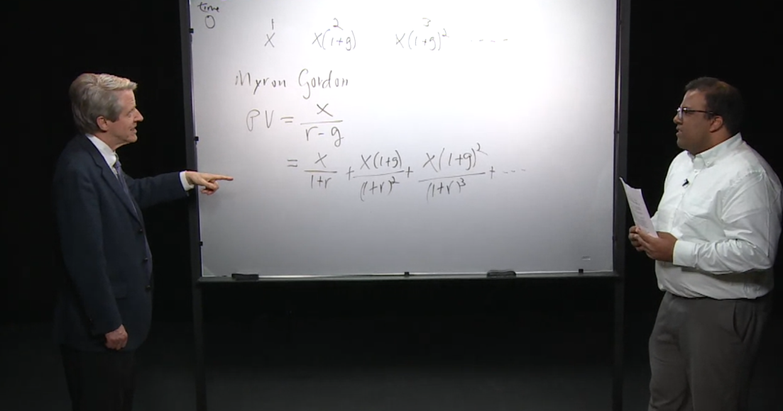
So, Professor, if I was hoping we can go through
the idea of the Gordon Growth Model? >> Mm-hm. >> And kind of how that relates
to what we’ve learned in CAPM? >> Myron Gordon, a half century ago,
nearly told what, he gave a formula for
the present value of a growing quantity. Suppose we have an asset,
let’s call it land, that is producing revenue for you every year, and
the revenue is growing in value. So it produces x the first year, then
it produces x times 1 + g growth rate, the next year, and
then it produces x times 1 + the growth rate squared the next year,
and then it does that forever. So this is year, now it’s times 0, and then we have time 1, time 2, times 3, time 4, it would be 1 + g cubed etc. I say this might be land, because land,
assuming that it’s managed properly and doesn’t get depleted,
will yield a crop every year. And as time goes on,
the crop will be worth more. Partly because demand for it probably
goes up in a growing economy and probably because of technical progress. And we’re going to assume this land
goes on growing like this forever.
So the question is what do you pay for
this land at time 0? Okay, so Myron Gordon, he’s famous for this formula principally, is that the present value = x/(r- g), where r is the rate of discount. What he’s saying is that, the present value is x/(1 + r), that’s this first term here,+ x (1 + g)/(1 + r squared) + x (1+g) squared/(1 + r cubed), okay. And if you calculate, you can show that infinite sum reduces to this simple formula, as long as g is less than r. If g is less than r, then each term
is smaller than the one before it. And it sums to a finite number. If g equals r,
then every term here is x/1 + r, they are all the same, and so
the sum would be infinite. So as long as g is less than r this
is a formula for pricing the value of a asset that actually yields
an infinite amount, but in the future It’s
actually growing forever. [LAUGH] Right, so
actually g can be negative also. It doesn’t matter whether it’s positive or
negative. >> So that would be like you’re losing
some proportion every [CROSSTALK] >> Yeah- >> Every decade or something. >> It could be that
the land is being depleted. >> Okay.
And so the growth rate of the value is negative. So then this becomes r plus
something because g is negative. You still have a present value, and
this is an important thing to recognize, that even assets whose payments
are running down to zero, there still is a price for them today. That’s really important to recognize. So some people think that businesses that
are growing are the only ones I should invest in. That’s bad investing. You can make a fortune investing
in businesses that are declining. You can fill up your portfolio
with declining industries. It doesn’t matter, it’s the question,
can you buy them for less than the present value? And if you’re buying them for less than
the present value, it’s a good investment. >> I see. And so, here, just to clarify, g is given? >> Yes, I’m taking that as given, the
growth rate, it might be like 2% a year. >> Right
And the interest, r might be 5% a year. >> Okay. >> The value would be x divided by
5% minus 2% or x divided by 0.03. >> Okay. >> And this is a very useful formula because a lot of possible
investments have a growth rate. In fact they usually do. Usually you don’t expect the earnings
of a company, for example, to stay exactly where they are today. Some companies are expected
to grow through time and some are expected to decline through time. So you end up using this
formula all the time to judge. You look at their earnings today and
you think, well what is it worth? What is the stream of
future earnings worth? And you can plug it into this formula. >> I see, and r is that also given or is that-
Now, okay. >> Being determined? >> Now I haven’t talked
about risk in this equation. I was saying the land is going to do this,
we just know this for certain. >> Right, that’s just given. >> But we don’t in fact, often,
we don’t know the future with certainty. So there’s an amount of risk. So if this growth rate is more
uncertain than you thought, that should lower the price. Right, so if the assets is riskless,
if there’s is no risk, if we actually know all the future payouts from the asset, then this r
would be the riskless interest rate. But if it’s greater, if there is risk. And that would be measured by beta
in the capital asset pricing model. Then r would be increased
reflecting that risk. You still use the same Gordon formula,
but you have a higher r. R is no longer the riskless rate. >> Okay. And I also found that to be a very
fascinating statement you made that even if most people I think
typically think that if there’s a industry that’s declining,
I don’t want to have that in my portfolio. >> Right.
But in this case we’re kind of bringing out the idea that even stocks of declining
industries, those should be in your portfolio if you kind of followed the-
Right.
The standard traditional [CROSSTALK]
I like to bring up the example of railroads. When the first railroads came in,
well it was in the 1830s, but by the 1840s,
there was a big bubble in railroad stocks. Lots of people thought wow,
railroads are growing. They were right. Railroads were growing. But people paid too much. Even though they’re growing,
you can pay more than the present value. So lots of famous people in the very
beginning of the railroad era, lost fortune, even including
Charles Darwin, the great biologist. He couldn’t figure out present value. He was a smart guy, but he couldn’t figure out what the real
value of these railroad stocks were. But then as time went on, railroads
stopped being glamorous and exciting. And they became old hat. And then we got airplanes, and trucks, and cars, and
all these other alternatives to railroads. So railroad stocks then became
underpriced relative to this formula. So one of the best investments
to make in 1929 was railroads, already people were thinking about Charles
Lindbergh flew across the Atlantic Ocean, everything is moving fast for airlines,
and they just got overpriced. The same thing happened in the year 2000. In 2000,
that was the peak of the dot-com bubble. Everybody was investing in computer or
software, or social media stocks. And because they saw the growth rate. But they made a mistake. You have to use this formula. They made a mistake in thinking that
they’re worth more than they really were, and the whole dot-com bubble collapsed. The good thing to invest in, if you
could go back in a time machine to 2000, was railroads,
[LAUGH] everyone was ignoring them. But they’re still chugging along,
doing all this work. And now, even being declining industry, it wasn’t living up to
expectations initially, in terms of earnings growth,
but they made good investments. Sometimes, not every time, depending on how the price compares to
the present value of their earnings.
教授讲解了Gordon增长模型(Gordon Growth Model),并讨论了它与资本资产定价模型(CAPM)的关系。以下是教授讲解的重点总结:
Gordon增长模型的基本概念
公式的背景:
- Myron Gordon提出了一个公式,用于计算一个不断增长的资产的现值。假设有一块土地,每年为你产生收益,并且收益逐年增长。
- 每年的收益可以表示为:第一年为x,第二年为x(1+g),第三年为x(1+g)^2,依此类推,收益会一直增长。
公式的推导:
- Gordon公式为:[ Present Value = x r − g \text{Present Value} = \frac{x}{r - g} Present Value=r−gx ]
- 其中,x是第一年的收益,r是贴现率,g是收益的增长率。
- 该公式表示,当增长率小于贴现率时,无限期增长的收益流的现值可以简化为这一公式。
公式的应用与限制
增长率与贴现率的关系:
- 如果增长率g大于或等于贴现率r,公式将无法应用,因为收益流的总和会变得无限大。
- 增长率g可以为负,表示收益在减少,这时公式变为[ $\text{Present Value} = \frac{x}{r + |g|} $],仍然有一个有限的现值。
风险的考虑:
- 公式假设未来收益是确定的,即没有风险。在现实中,未来收益通常是有不确定性的,因此需要考虑风险。
- 在考虑风险时,r需要调整为包含风险溢价的贴现率。这可以通过CAPM模型中的β来反映风险。
投资决策中的应用
错误的投资观念:
- 很多人认为只有不断增长的行业才值得投资,这是一个错误的观念。实际上,即使是处于衰退的行业,只要购买价格低于其现值,也是好的投资。
- 举例来说,在1929年和2000年的特定时期,铁路股票和其他被忽视的行业股票实际上是很好的投资机会,因为它们的价格低于其现值。
历史教训:
- 19世纪40年代的铁路股票泡沫和2000年的互联网泡沫都是因为投资者过高估计了这些行业的增长率,导致支付的价格高于现值,从而遭受损失。
- 反之,在这些行业不再被关注时,股票价格低于其现值,反而成为了好的投资机会。
总结
Gordon增长模型为我们提供了一个简单而有效的方法来估算持续增长资产的现值,但在应用时需要考虑增长率、贴现率和风险等因素。投资者不应只关注增长的行业,也应关注被低估的行业,关键在于所支付的价格是否低于其现值。
Sure, here’s a summary of the key points discussed by the professor regarding the Gordon Growth Model:
Basic Concepts of the Gordon Growth Model
Background of the Formula:
- Myron Gordon proposed a formula for calculating the present value of a perpetually growing asset. This formula is applicable to assets that generate increasing returns over time.
- The annual returns can be represented as follows: x for the first year, x(1+g) for the second year, x(1+g)^2 for the third year, and so on, where g represents the growth rate.
Derivation of the Formula:
- The Gordon formula is: [ Present Value = x r − g \text{Present Value} = \frac{x}{r - g} Present Value=r−gx ]
- Here, x is the return in the first year, r is the discount rate, and g is the growth rate of returns.
- The formula simplifies the infinite sum of growing returns under the assumption that the growth rate is less than the discount rate.
Application and Limitations of the Formula
Relation between Growth Rate and Discount Rate:
- If the growth rate g is greater than or equal to the discount rate r, the formula cannot be applied as the sum of returns becomes infinite.
- The growth rate g can be negative, indicating decreasing returns. In this case, the formula becomes [ Present Value = x r + ∣ g ∣ \text{Present Value} = \frac{x}{r + |g|} Present Value=r+∣g∣x ], still yielding a finite present value.
Consideration of Risk:
- The formula assumes certainty in future returns, implying no risk. However, in reality, future returns often involve uncertainty, necessitating consideration of risk.
- When considering risk, the discount rate r needs to be adjusted to incorporate a risk premium. This adjustment can be reflected using β from the Capital Asset Pricing Model (CAPM).
Application in Investment Decision Making
Misconceptions about Investment:
- Many people believe that only growing industries are worth investing in, which is a misconception. Even declining industries can be good investments if purchased at prices below their present value.
- Historical examples, such as the railroad stock bubble in the 1840s and the dot-com bubble in 2000, demonstrate the consequences of overestimating growth rates and paying prices exceeding present values.
Historical Lessons:
- The railroad stocks of the 19th century and overlooked industries during the dot-com bubble serve as lessons that even declining industries can present investment opportunities when their prices are below their present values.
Conclusion
The Gordon Growth Model offers a simple and effective method for estimating the present value of perpetually growing assets. However, its application requires consideration of factors such as growth rate, discount rate, and risk. Investors should not only focus on growing industries but also explore undervalued opportunities, ensuring that prices paid are below present values.
使用未来的收益计算现值(Present Value,PV)有重要的意义,特别是在财务和投资领域。这里有几个关键点解释为什么这种计算方法很有意义:
- 时间价值的概念
时间价值是金融学中的一个基本概念,它指出钱在不同的时间点的价值是不同的。一般来说,今天的一美元比未来的一美元更有价值。这是因为今天的一美元可以被投资并产生回报,而未来的一美元在今天则无法利用。计算现值有助于反映这一时间价值的差异。
- 决策支持
通过计算投资或项目的现值,投资者和企业可以更好地评估不同投资选项的可行性和回报率。现值计算使得投资者能够比较不同时点上的现金流,帮助他们做出更明智的决策。
- 风险评估
未来的收益和现金流通常是不确定的。现值计算可以结合折现率(包括风险调整),帮助投资者量化和考虑不确定性和风险。较高的风险通常意味着较高的折现率,从而降低未来现金流的现值。
- 资本预算
企业在进行资本预算时,会评估多个项目的现值,以确定哪些项目值得投资。通过比较不同项目的现值,企业可以确定哪些项目能够提供最大的价值和回报。
- 评估资产价值
现值计算是评估各种资产价值的重要方法,包括股票、债券、房地产和企业。通过将未来的现金流折现到现在,投资者可以估算这些资产在当前的公平市场价值。
例子
假设一个项目将在未来五年内每年产生10,000美元的收益。如果折现率是5%,我们可以使用现值公式计算这五年收益的现值:
[ P V = 10 , 000 ( 1 + 0.05 ) 1 + 10 , 000 ( 1 + 0.05 ) 2 + 10 , 000 ( 1 + 0.05 ) 3 + 10 , 000 ( 1 + 0.05 ) 4 + 10 , 000 ( 1 + 0.05 ) 5 PV = \frac{10,000}{(1+0.05)^1} + \frac{10,000}{(1+0.05)^2} + \frac{10,000}{(1+0.05)^3} + \frac{10,000}{(1+0.05)^4} + \frac{10,000}{(1+0.05)^5} PV=(1+0.05)110,000+(1+0.05)210,000+(1+0.05)310,000+(1+0.05)410,000+(1+0.05)510,000]
这种计算将告诉我们,未来五年的收益在今天值多少钱,从而帮助我们决定是否投资这个项目。
总结
计算未来收益的现值是财务和投资决策中不可或缺的一部分。它通过考虑时间价值、风险和不确定性,帮助投资者和企业评估和比较不同的投资选项,从而做出更合理、更有依据的决策。
Using the present value (PV) of future cash flows is significant for several reasons, particularly in finance and investment contexts. Here are the key points explaining why this calculation method is meaningful:
- Time Value of Money
The time value of money is a fundamental concept in finance, which states that money available today is worth more than the same amount in the future due to its potential earning capacity. This principle underlies the necessity to discount future cash flows to their present value, reflecting the idea that money now can be invested to generate returns.
- Informed Decision-Making
Calculating the present value of investments or projects helps investors and companies assess the feasibility and profitability of different options. By comparing cash flows at different times, they can make more informed decisions about where to allocate resources for the best return.
- Risk Assessment
Future earnings and cash flows are often uncertain. Present value calculations can incorporate discount rates that account for risk, allowing investors to quantify and consider uncertainty and risk. Higher risk typically results in a higher discount rate, which reduces the present value of future cash flows, reflecting the risk premium.
- Capital Budgeting
In capital budgeting, companies evaluate multiple projects by comparing their present values to determine which projects are worth pursuing. By comparing the present value of different projects, companies can identify those that offer the greatest value and return.
- Valuing Assets
Present value calculations are essential for valuing various assets, including stocks, bonds, real estate, and businesses. By discounting future cash flows to the present, investors can estimate the fair market value of these assets.
Example
Suppose a project will generate $10,000 in revenue each year for the next five years. If the discount rate is 5%, we can use the present value formula to calculate the present value of these five years of revenue:
[ P V = 10 , 000 ( 1 + 0.05 ) 1 + 10 , 000 ( 1 + 0.05 ) 2 + 10 , 000 ( 1 + 0.05 ) 3 + 10 , 000 ( 1 + 0.05 ) 4 + 10 , 000 ( 1 + 0.05 ) 5 PV = \frac{10,000}{(1+0.05)^1} + \frac{10,000}{(1+0.05)^2} + \frac{10,000}{(1+0.05)^3} + \frac{10,000}{(1+0.05)^4} + \frac{10,000}{(1+0.05)^5} PV=(1+0.05)110,000+(1+0.05)210,000+(1+0.05)310,000+(1+0.05)410,000+(1+0.05)510,000]
This calculation tells us how much those future revenues are worth today, helping us decide whether to invest in this project.
Conclusion
Calculating the present value of future earnings is a crucial aspect of financial and investment decision-making. It helps investors and companies evaluate and compare different investment options by considering the time value of money, risk, and uncertainty, leading to more rational and evidence-based decisions.
Lesson #4 Quiz
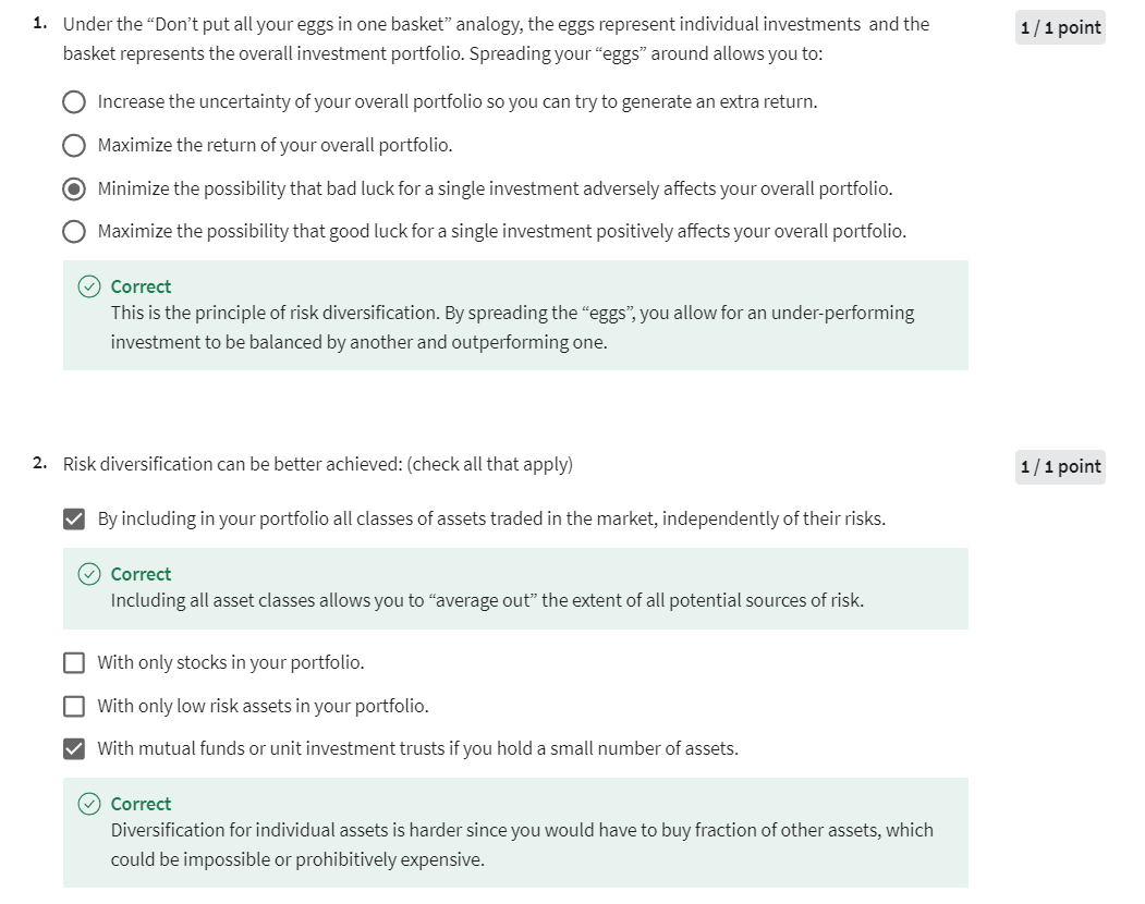
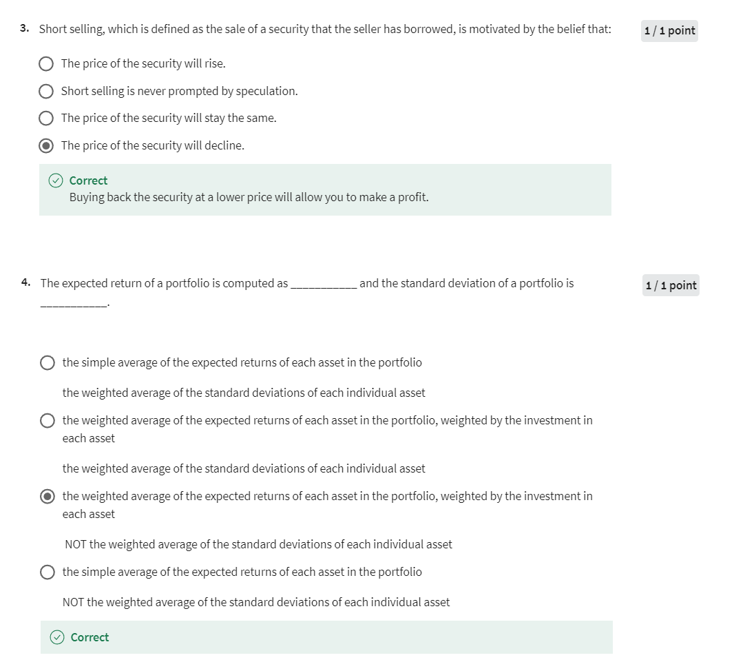
Module 1 Honors Quiz

Question 6
If an insurance company has 10000 policies, and each has 0.1 probability of making a claim, what is the standard deviation of the fraction of policies which result in a claim?
To calculate the standard deviation of the fraction of policies that result in a claim, we can use the properties of the binomial distribution. In this case, we have 10,000 policies and each policy has a probability of 0.1 of making a claim.
First, let’s define the variables:
- ( n = 10,000 ) (the number of policies)
- ( p = 0.1 ) (the probability of making a claim)
The number of claims, ( X ), follows a binomial distribution ( X ∼ Binomial ( n , p ) X \sim \text{Binomial}(n, p) X∼Binomial(n,p) ).
The mean ( μ \mu μ ) and standard deviation ( σ \sigma σ ) of a binomial distribution are given by:
[ μ = n p \mu = np μ=np ]
[ σ = n p ( 1 − p ) \sigma = \sqrt{np(1 - p)} σ=np(1−p) ]
However, we are interested in the standard deviation of the fraction of policies that result in a claim, which is ( X n \frac{X}{n} nX). To find this, we need to calculate the standard deviation of ( X ) and then divide by ( n ).
Calculate the mean number of claims:
[ μ = n p = 10 , 000 × 0.1 = 1 , 000 \mu = np = 10,000 \times 0.1 = 1,000 μ=np=10,000×0.1=1,000 ]Calculate the standard deviation of the number of claims:
[ σ X = n p ( 1 − p ) = 10 , 000 × 0.1 × 0.9 = 900 = 30 \sigma_X = \sqrt{np(1 - p)} = \sqrt{10,000 \times 0.1 \times 0.9} = \sqrt{900} = 30 σX=np(1−p)=10,000×0.1×0.9=900=30 ]The standard deviation of the fraction of policies that result in a claim is:
[ σ X n = σ X n = 30 10 , 000 = 0.003 \sigma_{\frac{X}{n}} = \frac{\sigma_X}{n} = \frac{30}{10,000} = 0.003 σnX=nσX=10,00030=0.003 ]
Therefore, the standard deviation of the fraction of policies which result in a claim is ( 0.003 ).
第七题选择too big to fail不对,选择 strengthen insurance industry也不对。
Question 7
Why was the National Association of Insurance Commissioners created?
0 / 1 point
To suggest laws that would prevent insurance corporations from becoming “too big to fail”
To suggest laws that would decentralize the insurance industry
To suggest laws that would decrease the complexity of insurance regulation
To suggest laws that would strengthen the insurance industry
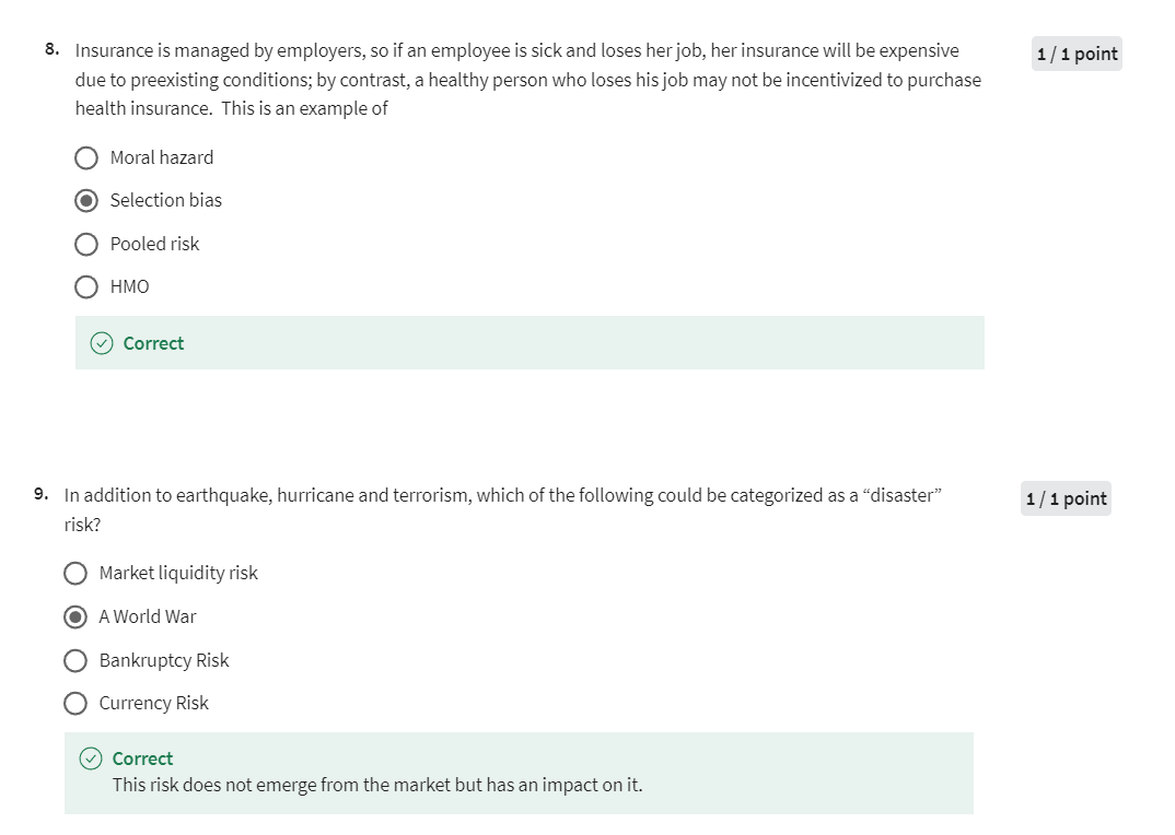
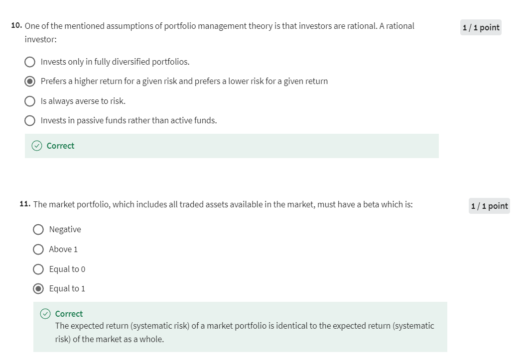
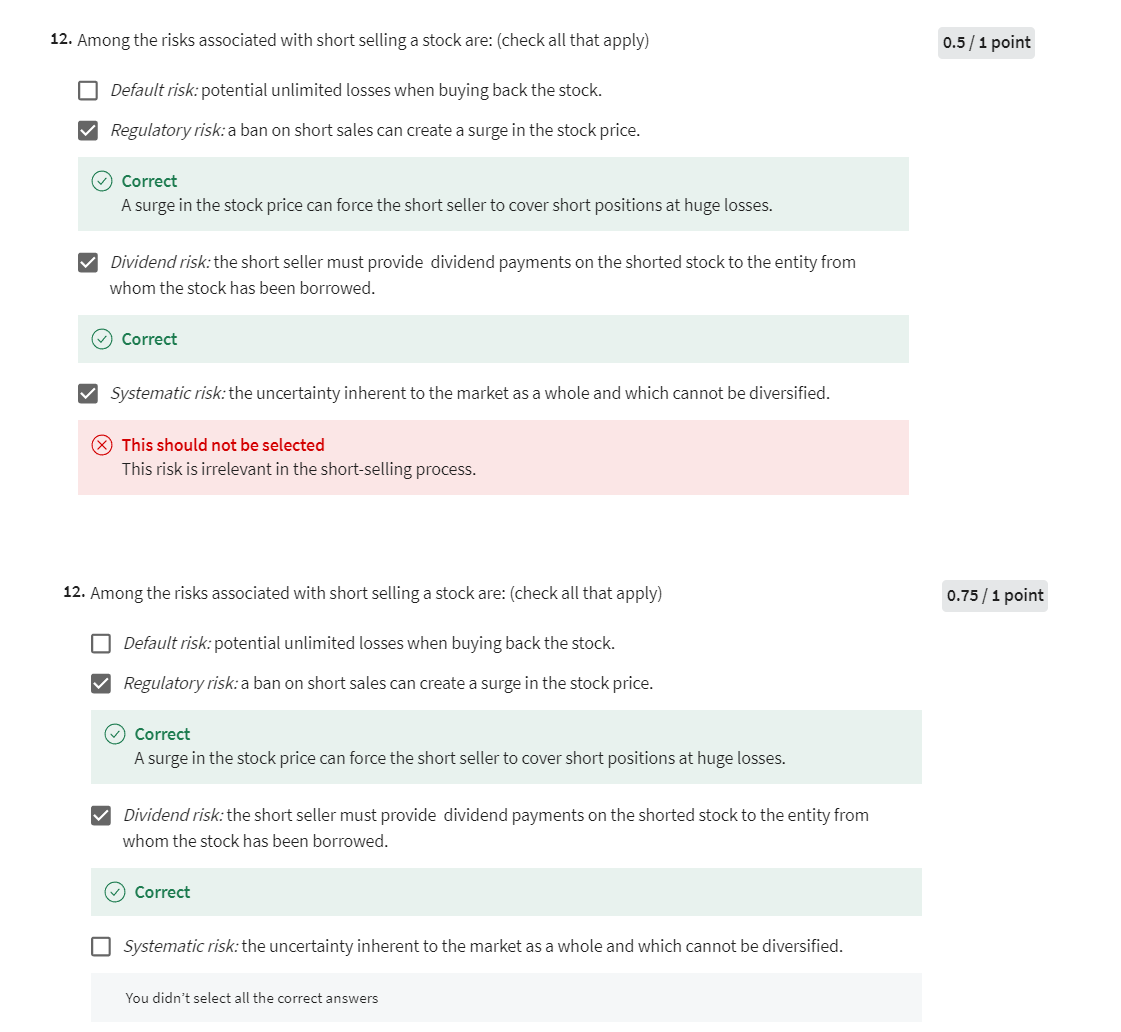
第12题选择前三个
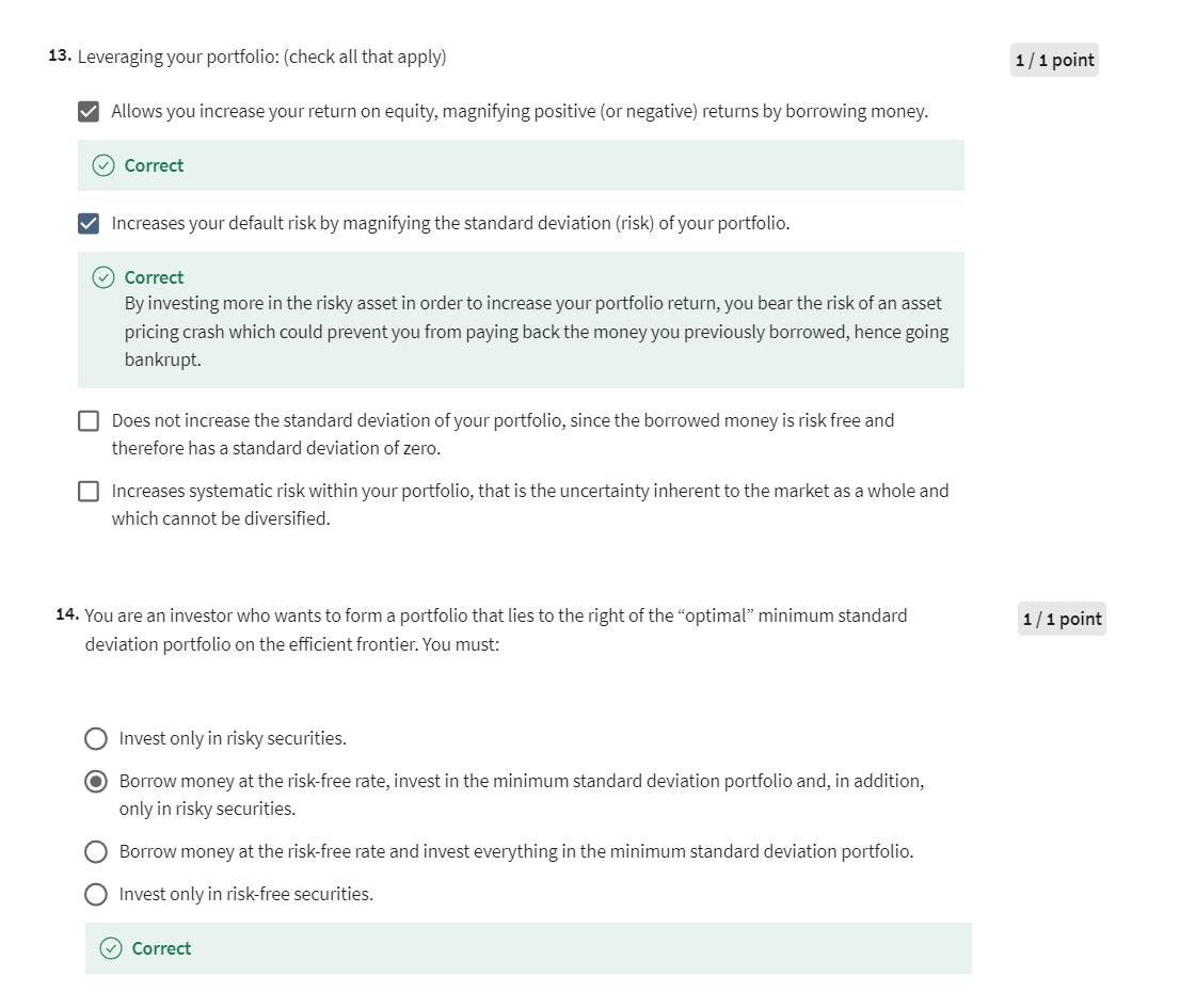
后记
2024年6月12日15点50分完成Week 1的学习。这位耶鲁大学的教授深入浅出,让我对之前的金融知识有了进一步的认识。由于我本科辅修过金融学专业,大多数概念我是了解的。在全英的环境下体验美国顶级名校的金融课程,终于自己的能力达到了不开字幕、倍速听英文课程的水平。希望自己的能力不断提升。