一、网络数据采集
证券宝是一个免费、开源的证券数据平台(无需注册),提供大盘准确、完整的证券历史行情数据、上市公司财务数据等,通过python API获取证券数据信息。
1. 安装并导入第三方依赖库 baostock
在命令提示符中运行:pip install baostock
导入依赖库
import baostock as bs
import pandas as ad
如果在安装anaconda之前有安装过Python,那么系统会把依赖库默认下载到之前的Python文件夹中,所以需要把旧路径添加到anaconda中。
import sys
sys.path.append("D:\Study Material\Python 3.13.0(64bit)\Lib\site-packages")
路径只需要添加一次
2. 登录系统
lg = bs.login()
# 显示登录返回信息
print(lg.error_code) # 错误代码,当为0时表示成功,当为非0时表示失败
print(lg.error_msg) # 错误信息,对错误的详细解释
结果:
login success!
0
success
3. 获取上证指数的历史数据
bs.query_history_k_data
分钟线指标:date,time,code,open,high,low,close,volume,amount,adjustflag
周月线指标:date,code,open,high,low,close,volume,amount,adjustflag,turn,pctChg
周月线详细指标参数:日期、代码、开盘价、最高价、最低价、收盘价、成交金额、复权情况、换手率、涨跌幅
rs = bs.query_history_k_data("sh.600000",
    "date,code,open,high,low,close,volume,amount,adjustflag,turn,pctChg",
    start_date='2021-05-23', end_date='2022-05-23',
    frequency="d", adjustflag="3")
print(rs.error_code)
print(rs.error_msg)
结果:
0
success
获取具体的信息:从rs中分页查询数据,将每页的数据合并到一个列表中,然后将这些数据转换为Pandas的DataFrame对象,最后将DataFrame保存为 CSV 文件并打印出来
result_list = []
while (rs.error_code == '0') & rs.next(): # 持续执行循环体中的代码,直到循环条件不满足为止
    # rs.next():如果存在下一行,则返回True,否则返回False
    # 判断错误码是否为'0'以及是否还有下一行数据。
    result_list.append(rs.get_row_data())
    # 调用rs对象的get_row_data方法获取当前行的数据并添加到list中
result = pd.DataFrame(result_list, columns=rs.fields)
# 将result_list列表转换为一个DataFrame对象
# columns=rs.fields:指定DataFrame的列名,rs.fields是一个包含列名的列表。
result.to_csv(".../history_k_data.csv", encoding="gbk", index=False)
# 调用DataFrame对象的to_csv方法将数据保存为CSV文件,index=False:表示不将DataFrame的索引保存到CSV文件中
print(result)
# 登出系统
bs.logout()
结果:
           date       code     open     high      low    close    volume  \
0    2021-05-24  sh.600000  10.0800  10.1400  10.0500  10.0900  23518901
1    2021-05-25  sh.600000  10.1000  10.3300  10.0600  10.3200  75417564
2    2021-05-26  sh.600000  10.3100  10.4200  10.2800  10.3500  54984815
3    2021-05-27  sh.600000  10.3200  10.4300  10.2600  10.2900  52063330
4    2021-05-28  sh.600000  10.3300  10.3600  10.2500  10.3500  34593293
..          ...        ...      ...      ...      ...      ...       ...
930  2025-03-25  sh.600000  10.6500  10.6900  10.5000  10.6100  37875416
931  2025-03-26  sh.600000  10.6000  10.6100  10.4500  10.4700  36660981
932  2025-03-27  sh.600000  10.5000  10.6600  10.4700  10.5500  42508671
933  2025-03-28  sh.600000  10.5300  10.5700  10.4100  10.4400  36572944
934  2025-03-31  sh.600000  10.4700  10.6300  10.3500  10.4300  49360687

             amount adjustflag      turn     pctChg
0    237130459.3700          3  0.080100   0.000000
1    771994298.4800          3  0.256900   2.279500
2    568991552.4000          3  0.187300   0.290700
3    536862488.3300          3  0.177400  -0.579700
4    356339747.2700          3  0.117900   0.583100
..              ...        ...       ...        ...
930  401332739.2900          3  0.129000   0.000000
931  385049553.5800          3  0.124900  -1.319500
932  449288518.5700          3  0.144800   0.764100
933  382165241.2900          3  0.124600  -1.042700
934  518371937.1300          3  0.168200  -0.095800

[935 rows x 11 columns]
logout success!
<baostock.data.resultset.ResultData at 0x2c815254310>
result
结果:
	  date	      code	      open	  high	 low	close	volume	      amount	adjustflag	turn	    pctChg
0	2021-05-24	sh.600000	10.0800	10.1400	10.0500	10.0900	23518901	237130459.3700	3	0.080100	0.000000
1	2021-05-25	sh.600000	10.1000	10.3300	10.0600	10.3200	75417564	771994298.4800	3	0.256900	2.279500
2	2021-05-26	sh.600000	10.3100	10.4200	10.2800	10.3500	54984815	568991552.4000	3	0.187300	0.290700
3	2021-05-27	sh.600000	10.3200	10.4300	10.2600	10.2900	52063330	536862488.3300	3	0.177400	-0.579700
4	2021-05-28	sh.600000	10.3300	10.3600	10.2500	10.3500	34593293	356339747.2700	3	0.117900	0.583100
...	...	...	...	...	...	...	...	...	...	...	...
930	2025-03-25	sh.600000	10.6500	10.6900	10.5000	10.6100	37875416	401332739.2900	3	0.129000	0.000000
931	2025-03-26	sh.600000	10.6000	10.6100	10.4500	10.4700	36660981	385049553.5800	3	0.124900	-1.319500
932	2025-03-27	sh.600000	10.5000	10.6600	10.4700	10.5500	42508671	449288518.5700	3	0.144800	0.764100
933	2025-03-28	sh.600000	10.5300	10.5700	10.4100	10.4400	36572944	382165241.2900	3	0.124600	-1.042700
934	2025-03-31	sh.600000	10.4700	10.6300	10.3500	10.4300	49360687	518371937.1300	3	0.168200	-0.095800
935 rows × 11 columns
4. 转换数据类型
# 数据类型为 字符串 str
print(type(result.open[0]))
# open[0]:获取可迭代对象中的第一个元素

# 去掉 date code adjustflag 列
data = result.drop(['date', 'code', 'adjustflag'], axis =1)
# axis=1:按列操作;axis=0:按行操作

# 将数据类型转为 数值 float 类型
for i in data.columns: data.loc[:,i] = pd.to_numeric(data.loc[:,i],errors = 'coerce')
data
'''
data.columns 是一个包含 data 这个 DataFrame 所有列名的索引对象
i 会依次代表 data 中的每一个列名,从而可以对每一列的数据进行操作。
data.loc 是 Pandas 里用于基于标签进行索引的方法。
data.loc[:,i] 表示选择 data 中列名为 i 的整列数据。
pd.to_numeric() 是 Pandas 提供的用于转换为数值类型的一个函数。
errors = 'coerce' 是一个参数设置,它表明在转换过程中,如果遇到无法转换为数值的值,就会将这些值强制转换为 NaN。
'''
print(type(data.open[0]))
结果:
<class 'str'>
    open	high	low	    close	volume	      amount	     turn	pctChg
0	10.08	10.14	10.05	10.09	23518901	2.371305e+08	0.0801	0.0000
1	10.10	10.33	10.06	10.32	75417564	7.719943e+08	0.2569	2.2795
2	10.31	10.42	10.28	10.35	54984815	5.689916e+08	0.1873	0.2907
3	10.32	10.43	10.26	10.29	52063330	5.368625e+08	0.1774	-0.5797
4	10.33	10.36	10.25	10.35	34593293	3.563397e+08	0.1179	0.5831
...	...	...	...	...	...	...	...	...
930	10.65	10.69	10.50	10.61	37875416	4.013327e+08	0.1290	0.0000
931	10.60	10.61	10.45	10.47	36660981	3.850496e+08	0.1249	-1.3195
932	10.50	10.66	10.47	10.55	42508671	4.492885e+08	0.1448	0.7641
933	10.53	10.57	10.41	10.44	36572944	3.821652e+08	0.1246	-1.0427
934	10.47	10.63	10.35	10.43	49360687	5.183719e+08	0.1682	-0.0958
935 rows × 8 columns
<class 'numpy.float64'>
# 最后一列 涨跌幅 pctChg 用 0-1 代替,1:涨,0:未涨
import numpy as np
data.pctChg = (data.pctChg>0)*1
data.to_csv(".../sh600000.csv", encoding="gbk", index=False)
data
'''
data.pctChg 表示访问 data 数据框中的 pctChg 列。
data.pctChg > 0 是一个布尔表达式,会对 pctChg 列中的每个元素进行比较,判断其是否大于 0。比较结果是一个布尔类型的 Series,其中大于 0 的元素对应的位置为 True,小于等于 0 的元素对应的位置为 False。
(data.pctChg > 0) * 1 会将布尔类型的 Series 转换为数值类型的 Series,True 转换为 1,False 转换为 0。
最后,将转换后的 Series 重新赋值给 data.pctChg,实现了对 pctChg 列的二值化处理。
'''
结果:
     open	 high	 low	close	 volume	      amount	     turn	pctChg
0	10.08	10.14	10.05	10.09	23518901	2.371305e+08	0.0801	0
1	10.10	10.33	10.06	10.32	75417564	7.719943e+08	0.2569	1
2	10.31	10.42	10.28	10.35	54984815	5.689916e+08	0.1873	1
3	10.32	10.43	10.26	10.29	52063330	5.368625e+08	0.1774	0
4	10.33	10.36	10.25	10.35	34593293	3.563397e+08	0.1179	1
...	...	...	...	...	...	...	...	...
930	10.65	10.69	10.50	10.61	37875416	4.013327e+08	0.1290	0
931	10.60	10.61	10.45	10.47	36660981	3.850496e+08	0.1249	0
932	10.50	10.66	10.47	10.55	42508671	4.492885e+08	0.1448	1
933	10.53	10.57	10.41	10.44	36572944	3.821652e+08	0.1246	0
934	10.47	10.63	10.35	10.43	49360687	5.183719e+08	0.1682	0
935 rows × 8 columns
二、KNN分类和预测
(一)划分训练集和测试集
# 前0.8数据作为训练集,后0.2数据作为测试集
# 前7个属性作为样本,最后一列作为标签
X = data.iloc[:,:-1] # 特征矩阵X
y = data.iloc[:,-1] # 目标向量y
# 借助iloc方法对data进行切片操作,选取所有行以及除最后一列之外的所有列

from sklearn.model_selection import train_test_split
X_train, X_test, y_train, y_test = train_test_split(X, y, test_size=0.20)
X_train, y_train, X_test, y_test # 输出四个对象,在实际应用中通常不会这么做
'''
从sklearn.model_selection模块里导入train_test_split函数,该函数可用于把数据集划分成训练集和测试集。
test_size=0.20:表明测试集在整个数据集中所占的比例为20%,那么训练集占比就是80%。
函数返回四个对象:
X_train:训练集的特征矩阵。
X_test:测试集的特征矩阵。
y_train:训练集的目标向量。
y_test:测试集的目标向量。
'''
结果:
(      open   high    low  close     volume        amount    turn
 148   8.56   8.59   8.54   8.57   29833707  2.555905e+08  0.1016
 502   7.43   7.49   7.39   7.45   20936996  1.557060e+08  0.0713
 612   6.92   6.92   6.86   6.87   18249280  1.254957e+08  0.0622
 268   8.05   8.06   8.00   8.01   23369617  1.876911e+08  0.0796
 513   7.30   7.33   7.23   7.28   17447358  1.268417e+08  0.0594
 ..     ...    ...    ...    ...        ...           ...     ...
 821  10.31  10.54  10.25  10.40   88307795  9.184083e+08  0.3009
 474   7.77   8.17   7.76   8.07  143117862  1.148390e+09  0.4876
 74    9.22   9.31   9.20   9.21   35627742  3.295036e+08  0.1214
 260   7.95   7.98   7.91   7.91   30065154  2.383203e+08  0.1024
 76    9.34   9.39   9.29   9.34   40941784  3.820179e+08  0.1395

 [748 rows x 7 columns],
 148    1
 502    1
 612    0
 268    0
 513    0
       ..
 821    1
 474    1
 74     0
 260    0
 76     0
 Name: pctChg, Length: 748, dtype: int32,
       open   high    low  close    volume        amount    turn
 351   6.70   6.74   6.66   6.71  24034116  1.608915e+08  0.0819
 458   7.23   7.23   7.18   7.18  20191251  1.453580e+08  0.0688
 235   7.91   8.05   7.90   8.05  37343358  2.989415e+08  0.1272
 34    9.96   9.99   9.90   9.91  33415612  3.322191e+08  0.1138
 829  10.12  10.25  10.12  10.14  24017341  2.443456e+08  0.0818
 ..     ...    ...    ...    ...       ...           ...     ...
 173   8.64   8.71   8.62   8.64  36223235  3.138612e+08  0.1234
 809   8.37   8.53   8.30   8.52  39163824  3.307787e+08  0.1334
 550   7.03   7.06   6.98   6.99  24604979  1.724132e+08  0.0838
 151   8.54   8.57   8.53   8.53  22929621  1.959416e+08  0.0781
 228   7.98   8.06   7.86   8.03  44512846  3.542461e+08  0.1517

 [187 rows x 7 columns],
 351    0
 458    0
 235    1
 34     0
 829    0
       ..
 173    0
 809    1
 550    0
 151    0
 228    1
 Name: pctChg, Length: 187, dtype: int32)
(二)利用KNN算法进行分类并评估
from sklearn.neighbors import KNeighborsClassifier
# 从sklearn.neighbors模块中导入KNeighborsClassifier类,该类用于实现 K 近邻分类算法
knn = KNeighborsClassifier(n_neighbors = 5)  # 定义KNN分类器
# 在进行分类时,会考虑最近的 5 个邻居的类别来决定当前样本的类别。
knn.fit(X_train, y_train) # 训练集训练
# 调用knn对象的fit方法,使用训练集的特征矩阵X_train和目标向量y_train对 KNN 模型进行训练。训练过程中,模型会学习训练数据的特征和对应的类别标签之间的关系。
y_pred = knn.predict(X_test) # 测试集预测
# 调用knn对象的predict方法,使用训练好的模型对测试集的特征矩阵X_test进行预测,得到预测的类别标签y_pred。

# 比较预测结果和真实结果
from sklearn.metrics import classification_report, confusion_matrix
# 从sklearn.metrics模块中导入classification_report和confusion_matrix函数,这两个函数用于评估分类模型的性能。
print(confusion_matrix(y_test, y_pred))  # 混淆矩阵
print(classification_report(y_test, y_pred)) # 预测结果
print() # 分隔输出
'''
混淆矩阵可以直观地展示模型在每个类别上的预测情况,包括真正例(True Positives)、假正例(False Positives)、真反例(True Negatives)和假反例(False Negatives)。
分类报告包含了每个类别的精确率(Precision)、召回率(Recall)、F1 值(F1-score)和支持度(Support),以及宏平均(Macro Average)和加权平均(Weighted Average)等指标。
macro avg 为列均值
weighted avg 为以类别样本占总样本比例为权重的加权平均
'''

x=range(41)
x[0]
'''
range() 函数用于创建一个不可变的整数序列,其语法为 range(start, stop, step),若只传入一个参数,那么 start 默认为 0,step 默认为 1。
x 是一个从 0 到 40 的整数序列。当使用 x[0] 时,是在获取这个序列的第一个元素。因为序列从 0 开始计数,所以第一个元素的值为 0。
'''
结果:
[[49 52]
 [53 33]]
                precision    recall  f1-score   support

           0       0.48      0.49      0.48       101
           1       0.39      0.38      0.39        86

    accuracy                           0.44       187
   macro avg       0.43      0.43      0.43       187
weighted avg       0.44      0.44      0.44       187

0
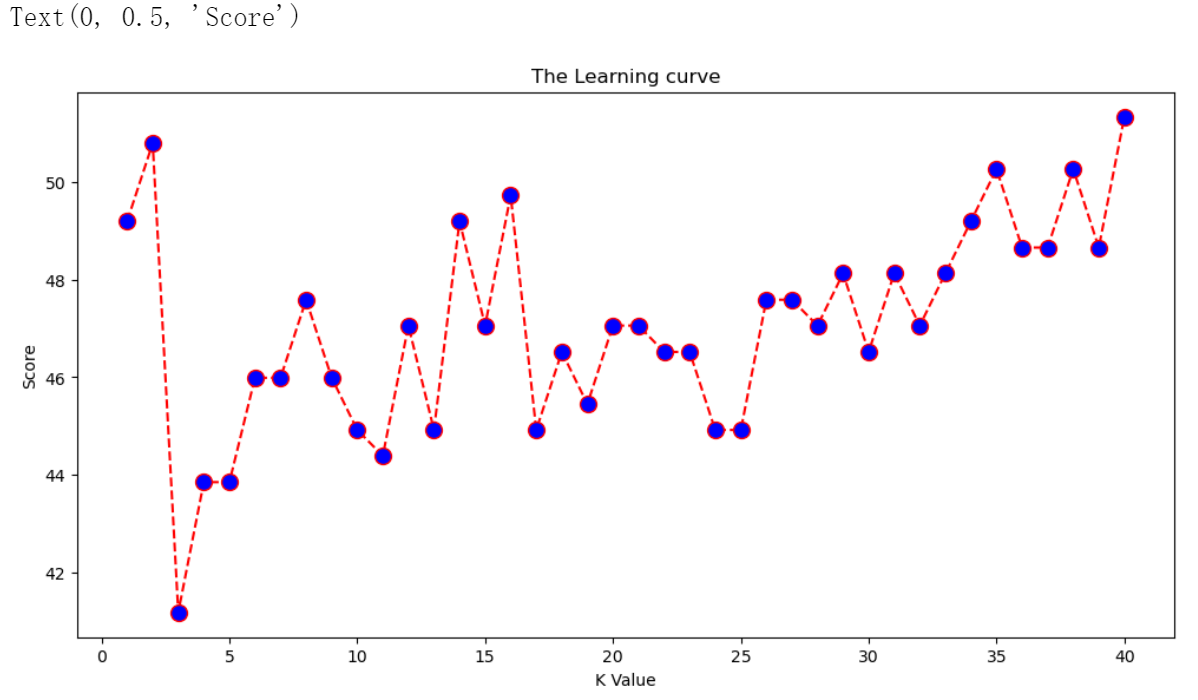
(三)改变 K 取值,绘制学习曲线
from sklearn.metrics import accuracy_score
import matplotlib.pyplot as plt
'''
从 sklearn.metrics 模块导入 accuracy_score 函数,该函数用于计算分类模型预测结果的准确率。
导入 matplotlib.pyplot 库,matplotlib 是 Python 中常用的绘图库。
'''

score = []
for K in range(40):
    K_value = K+1
    # range(40)生成的是从0到39的整数,加1得到1到40的K值
    knn = KNeighborsClassifier(n_neighbors = K_value)
    # 创建一个KNeighborsClassifier对象knn,并指定n_neighbors参数为当前的K_value。
    knn.fit(X_train, y_train) # 训练模型
    y_pred = knn.predict(X_test)
    # 使用训练好的模型对测试集的特征矩阵X_test进行预测,得到预测的类别标签y_pred。
    score.append(round(accuracy_score(y_test,y_pred)*100,2))
    # 计算预测结果的准确率,并将其乘以100转换为百分比形式,然后使用round函数保留两位小数,最后将结果添加到score列表中

plt.figure(figsize=(12, 6))  # 创建一个新的图形窗口,并设置图形的大小为宽12英寸,高6英寸。
plt.plot(range(1, 41), score, color='red', linestyle='dashed', marker='o',
         markerfacecolor='blue', markersize=10)
'''
使用 plt.plot 函数绘制学习曲线。
range(1, 41):作为 x 轴的数据,表示 K 的取值范围从 1 到 40。
score:作为 y 轴的数据,表示不同 K 值下模型在测试集上的准确率。
color='red':设置曲线的颜色为红色。
linestyle='dashed':设置曲线的样式为虚线。
marker='o':设置曲线上的数据点为圆形。
markerfacecolor='blue':设置数据点的填充颜色为蓝色。
markersize=10:设置数据点的大小为 10。
'''
plt.title('The Learning curve')  # 为图形添加标题
plt.xlabel('K Value')  # 为x轴添加标签
plt.ylabel('Score') # 为y轴添加标签
结果:
(四)最优K值的选择
error = []
# 计算K值在1-40之间多误差值
for i in range(1, 40):
    knn = KNeighborsClassifier(n_neighbors=i) # 设置参数
    knn.fit(X_train, y_train) # 训练模型
    pred_i = knn.predict(X_test) # 预测
    error.append(np.mean(pred_i != y_test))
    # 计算预测结果与真实标签不一致的比例(即误差率),np.mean函数用来计算平均值。

plt.figure(figsize=(12, 6))
plt.plot(range(1, 40), error, color='red', linestyle='dashed', marker='o',
         markerfacecolor='blue', markersize=10)
plt.title('Error Rate K Value')
plt.xlabel('K Value')
plt.ylabel('Mean Error')
结果:
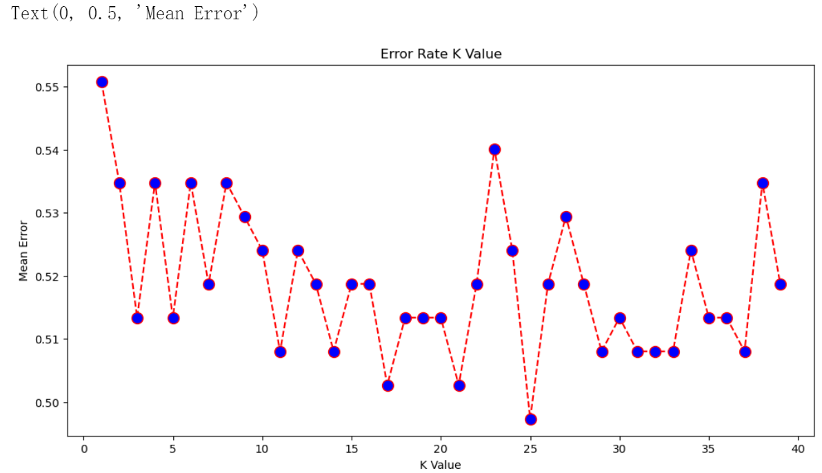
根据 score 和 error 来看,K=2 或 30 时,预测更准确
knn = KNeighborsClassifier(n_neighbors = 2)  # 定义KNN分类器
knn.fit(X_train, y_train) # 训练集训练
y_pred = knn.predict(X_test) # 测试集预测
# 比较预测结果和真实结果
from sklearn.metrics import classification_report, confusion_matrix
print(confusion_matrix(y_test, y_pred))  # 混淆矩阵
print(classification_report(y_test, y_pred)) # 预测结果

knn = KNeighborsClassifier(n_neighbors = 30)  # 定义KNN分类器
knn.fit(X_train, y_train) # 训练集训练
y_pred = knn.predict(X_test) # 测试集预测
# 比较预测结果和真实结果
from sklearn.metrics import classification_report, confusion_matrix
print(confusion_matrix(y_test, y_pred))  # 混淆矩阵
print(classification_report(y_test, y_pred)) # 预测结果
结果:
K=2时
[[67 24]
 [76 20]]
              precision    recall  f1-score   support

           0       0.47      0.74      0.57        91
           1       0.45      0.21      0.29        96

    accuracy                           0.47       187
   macro avg       0.46      0.47      0.43       187
weighted avg       0.46      0.47      0.43       187
K=10时
[[65 26]
 [70 26]]
              precision    recall  f1-score   support

           0       0.48      0.71      0.58        91
           1       0.50      0.27      0.35        96

    accuracy                           0.49       187
   macro avg       0.49      0.49      0.46       187
weighted avg       0.49      0.49      0.46       187
(五)用上面7个特征预测第二天的涨跌
对数据集 data 进行处理,去除最后一行和最后一列,然后根据 close 列的数据计算第二天是否上涨,并将结果添加为新列 up,最后将处理后的数据保存为 CSV 文件。
data
data1=data.iloc[:-1,:-1].copy() # 去掉最后一行和最后一列
data1['up']=((np.array(data.close[1:])-np.array(data.close[:-1]))>0)*1
'''
添加一列 up ,第二天是否上涨
由于iloc切片操作返回的是视图,为了避免后续修改data1时影响原始的data,使用copy()方法创建一个独立的副本。
np.array(data.close[1:]):将 data 数据框中 close 列从第二行开始的数据转换为 NumPy 数组
作差得到相邻两天close价格的差值,然后判断是否大于0,之后把布尔值转换为整数数组(*1)
data1['up']:计算结果作为新列'up',添加到data1中
'''
data1.to_csv(".../sh600000.csv", encoding="gbk", index=False)
# 将data1保存为CSV文件,不将数据框的索引保存到 CSV 文件中。
data1
结果:
	open	high	low	    close	volume	     amount	       turn	pctChg
0	10.08	10.14	10.05	10.09	23518901	2.371305e+08	0.0801	0
1	10.10	10.33	10.06	10.32	75417564	7.719943e+08	0.2569	1
2	10.31	10.42	10.28	10.35	54984815	5.689916e+08	0.1873	1
3	10.32	10.43	10.26	10.29	52063330	5.368625e+08	0.1774	0
4	10.33	10.36	10.25	10.35	34593293	3.563397e+08	0.1179	1
...	...	...	...	...	...	...	...	...
930	10.65	10.69	10.50	10.61	37875416	4.013327e+08	0.1290	0
931	10.60	10.61	10.45	10.47	36660981	3.850496e+08	0.1249	0
932	10.50	10.66	10.47	10.55	42508671	4.492885e+08	0.1448	1
933	10.53	10.57	10.41	10.44	36572944	3.821652e+08	0.1246	0
934	10.47	10.63	10.35	10.43	49360687	5.183719e+08	0.1682	0
935 rows × 8 columns

	open	high	low	    close	volume	      amount	     turn	up
0	10.08	10.14	10.05	10.09	23518901	2.371305e+08	0.0801	1
1	10.10	10.33	10.06	10.32	75417564	7.719943e+08	0.2569	1
2	10.31	10.42	10.28	10.35	54984815	5.689916e+08	0.1873	0
3	10.32	10.43	10.26	10.29	52063330	5.368625e+08	0.1774	1
4	10.33	10.36	10.25	10.35	34593293	3.563397e+08	0.1179	0
...	...	...	...	...	...	...	...	...
929	10.42	10.63	10.42	10.61	46449659	4.895272e+08	0.1582	0
930	10.65	10.69	10.50	10.61	37875416	4.013327e+08	0.1290	0
931	10.60	10.61	10.45	10.47	36660981	3.850496e+08	0.1249	1
932	10.50	10.66	10.47	10.55	42508671	4.492885e+08	0.1448	0
933	10.53	10.57	10.41	10.44	36572944	3.821652e+08	0.1246	0
934 rows × 8 columns
# 前7个属性作为样本,最后一列作为标签
X = data1.iloc[:,:-1]
y = data1.iloc[:,-1]

# 前0.8数据作为训练集,后0.2数据作为测试集
from sklearn.model_selection import train_test_split
from sklearn.preprocessing import StandardScaler
X_train, X_test, y_train, y_test = train_test_split(X, y, test_size=0.20)

# 标准化
scaler = StandardScaler()
scaler.fit(X_train)
X_train = scaler.transform(X_train)
X_test = scaler.transform(X_test)

# 改变 K 取值,比较错误率
error = []

# 计算K值在1-40之间多误差值
for i in range(1, 40):
    knn = KNeighborsClassifier(n_neighbors=i)
    knn.fit(X_train, y_train)
    pred_i = knn.predict(X_test)
    error.append(np.mean(pred_i != y_test))
plt.figure(figsize=(12, 6))
plt.plot(range(1, 40), error, color='red', linestyle='dashed', marker='o',
         markerfacecolor='blue', markersize=10)
plt.title('Error Rate K Value')
plt.xlabel('K Value')
plt.ylabel('Mean Error')
结果:
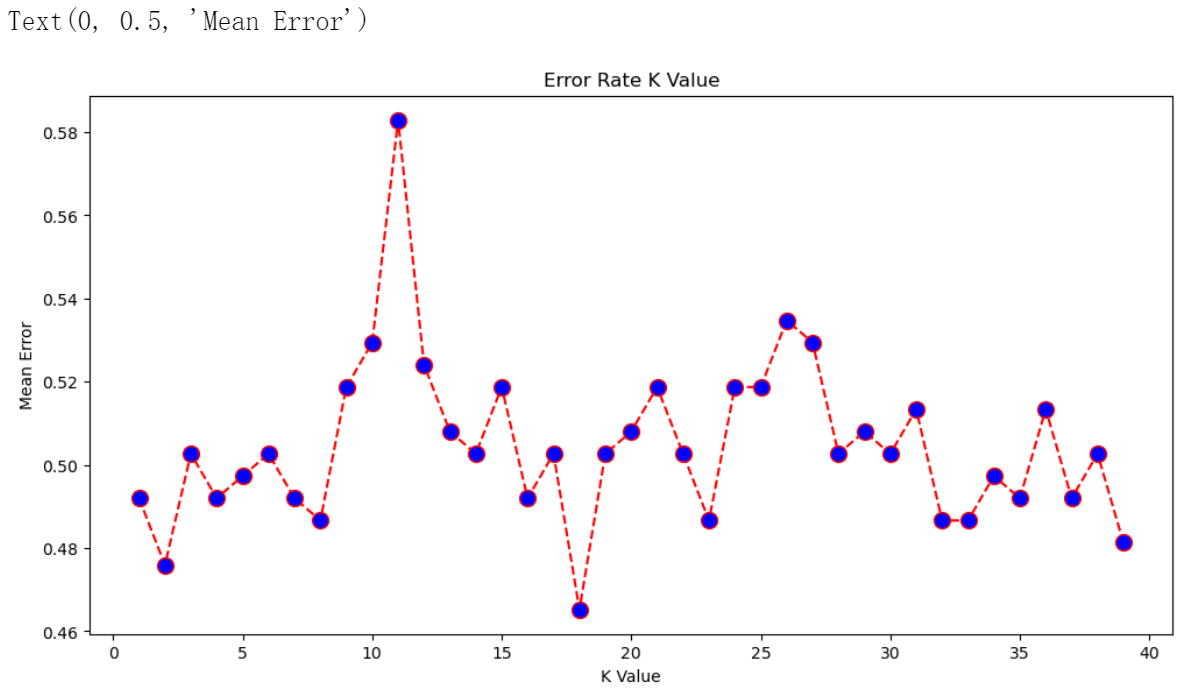
# 取 K = 29
knn = KNeighborsClassifier(n_neighbors = 29)  # 定义KNN分类器
knn.fit(X_train, y_train) # 训练集训练
y_pred = knn.predict(X_test) # 测试集预测

# 比较预测结果和真实结果
print(confusion_matrix(y_test, y_pred))  # 混淆矩阵
print(classification_report(y_test, y_pred)) # 预测结果
结果:
[[60 45]
 [50 32]]
              precision    recall  f1-score   support

           0       0.55      0.57      0.56       105
           1       0.42      0.39      0.40        82

    accuracy                           0.49       187
   macro avg       0.48      0.48      0.48       187
weighted avg       0.49      0.49      0.49       187
预测精确率为 57%
(六)鸢尾花数据
from sklearn import datasets # 提供示例数据集
import pandas as pd # 用于数据处理和分析的强大库
import numpy as np # 于科学计算的基础库,提供了高效的数组操作功能
import matplotlib # 常用的绘图库
import matplotlib.pyplot as plt # 提供了类似 MATLAB 的绘图接口

iris = datasets.load_iris() # 鸢尾花数据
# 调用datasets模块中的load_iris函数来加载鸢尾花数据集,返回一个包含数据集信息的字典对象,将其赋值给变量 iris

# 前0.8数据作为训练集,后0.2数据作为测试集
from sklearn.model_selection import train_test_split
X_train, X_test, y_train, y_test = train_test_split(iris.data, iris.target, test_size=0.20)

# 标准化
scaler = StandardScaler()
scaler.fit(X_train)
X_train = scaler.transform(X_train)
X_test = scaler.transform(X_test)

# 改变 K 取值,比较错误率
error = []

# 计算K值在1-40之间多误差值
for i in range(1, 40):
    knn = KNeighborsClassifier(n_neighbors=i)
    knn.fit(X_train, y_train)
    pred_i = knn.predict(X_test)
    error.append(np.mean(pred_i != y_test))
plt.figure(figsize=(12, 6))
plt.plot(range(1, 40), error, color='red', linestyle='dashed', marker='o',
         markerfacecolor='blue', markersize=10)
plt.title('Error Rate K Value')
plt.xlabel('K Value')
plt.ylabel('Mean Error')
结果:
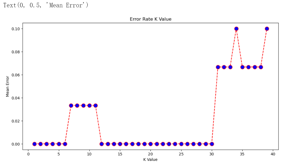
# 取 K = 5
knn = KNeighborsClassifier(n_neighbors = 5)  # 定义KNN分类器
knn.fit(X_train, y_train) # 训练集训练
y_pred = knn.predict(X_test) # 测试集预测

# 比较预测结果和真实结果
print(confusion_matrix(y_test, y_pred))  # 混淆矩阵
print(classification_report(y_test, y_pred)) # 预测结果
结果:
[[10  0  0]
 [ 0 13  0]
 [ 0  0  7]]
              precision    recall  f1-score   support

           0       1.00      1.00      1.00        10
           1       1.00      1.00      1.00        13
           2       1.00      1.00      1.00         7

    accuracy                           1.00        30
   macro avg       1.00      1.00      1.00        30
weighted avg       1.00      1.00      1.00        30
预测精度为 100%