分类问题之逻辑回归-EW帮帮网

什么是逻辑回归

逻辑回归实战准备

逻辑回归分类-考试通过预测

一阶线性模型

什么是逻辑回归

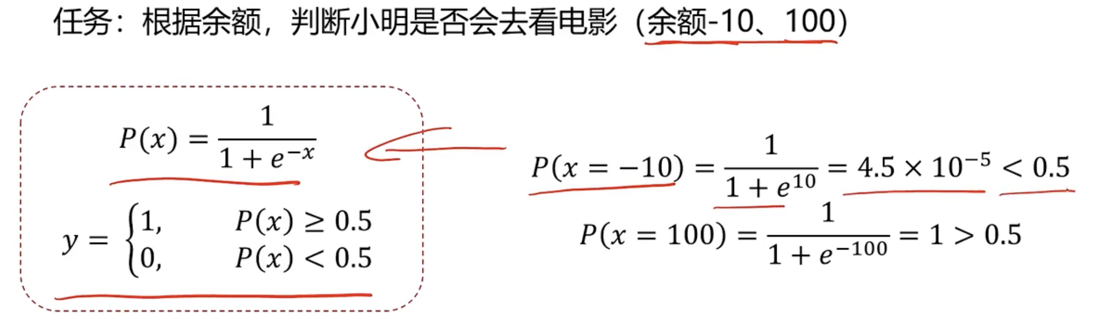
学习笔记：逻辑回归是属于分类问题，那如何去求解分类问题呢。假设是否去看电影，这里只是假设是否回去看电影

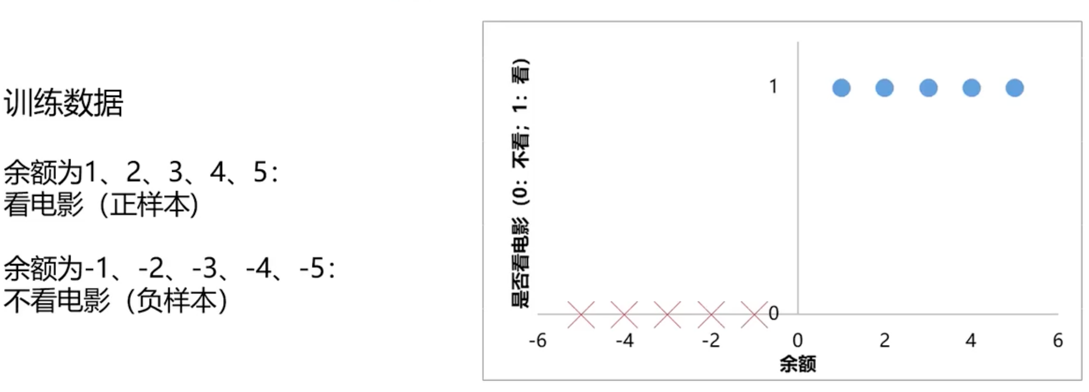
如果有钱就去消费，如果你还有房贷，车贷，各种欠款，可能就不会再去追求精神消费了

任务：根据余额，判断是否会去看电影，所以分类任务基本框架

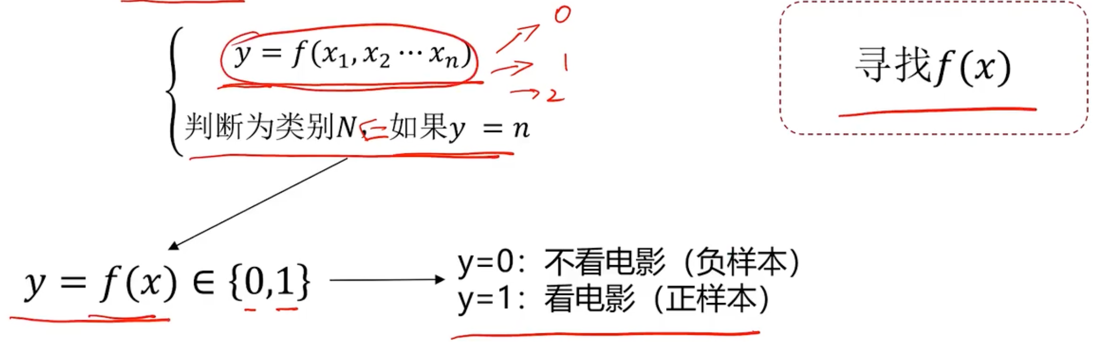
最简单的就是使用线性回归问题去判断下去找f(x)

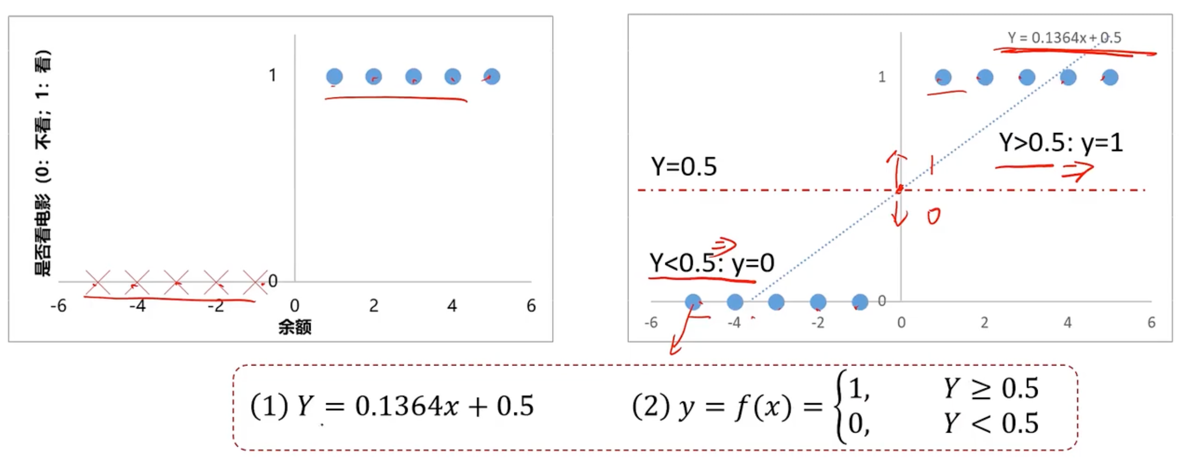
接着使用这个模型进行预测

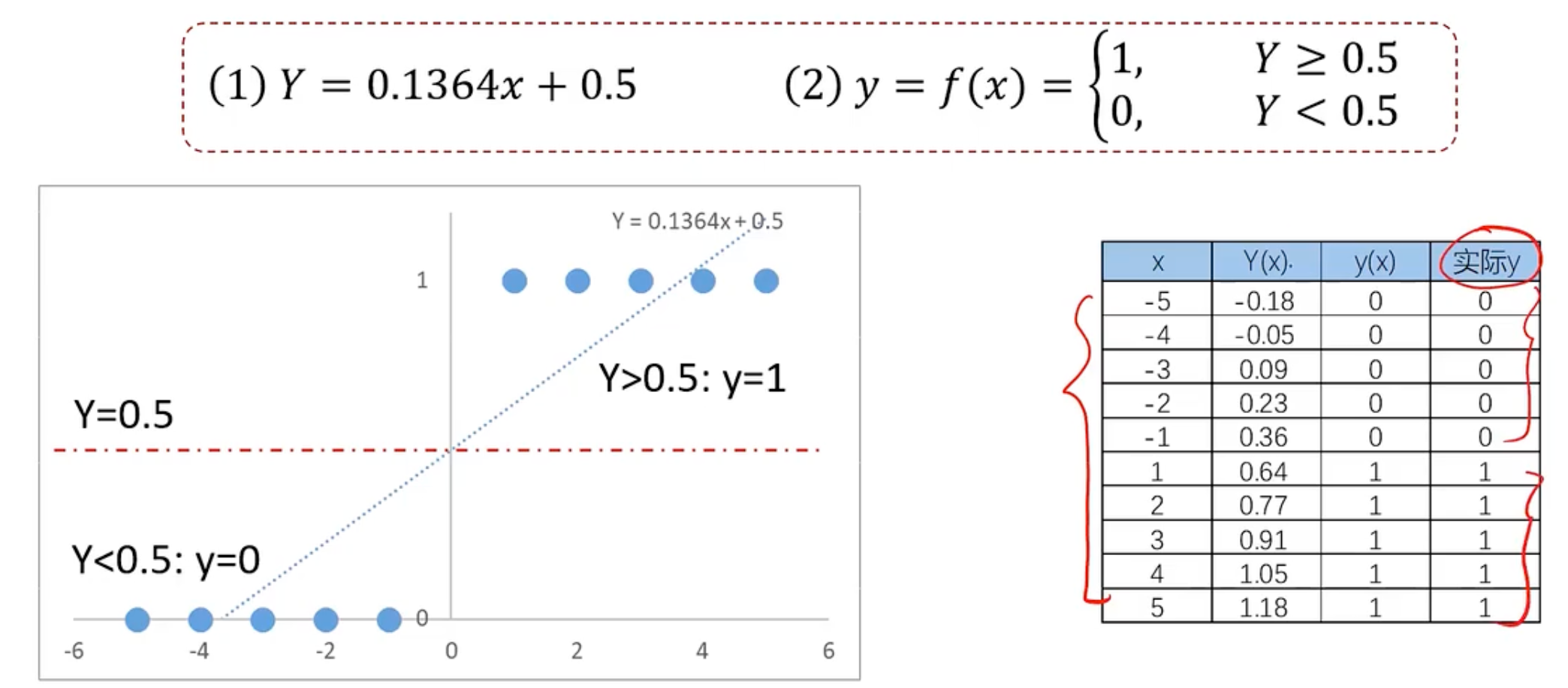
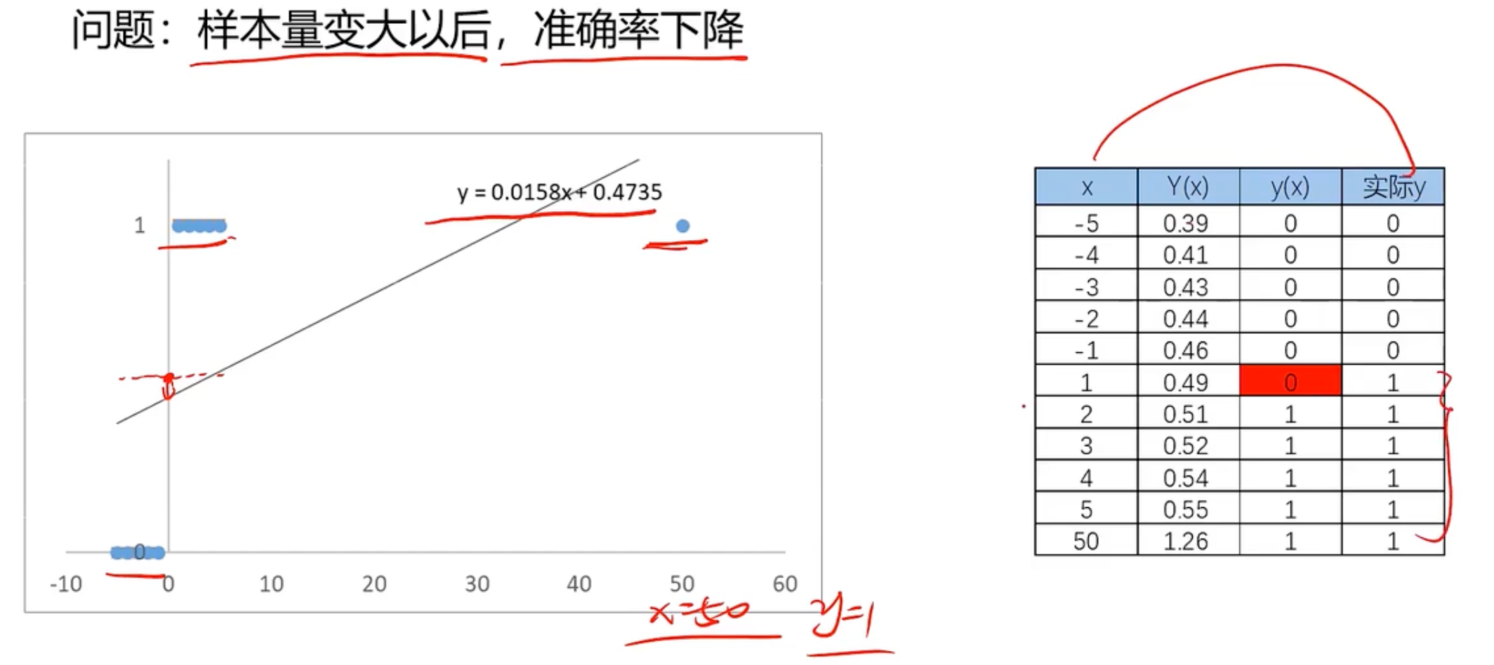
发现这样好像准确率还是可以的。那为什么不用这个呢？我们用下面的示例。就是x距离原点变远的时候，预测就开始不准确

所以我们此时需要一个新的更好的能用来分类的模型，称之为逻辑回归，逻辑回归方程如下所示

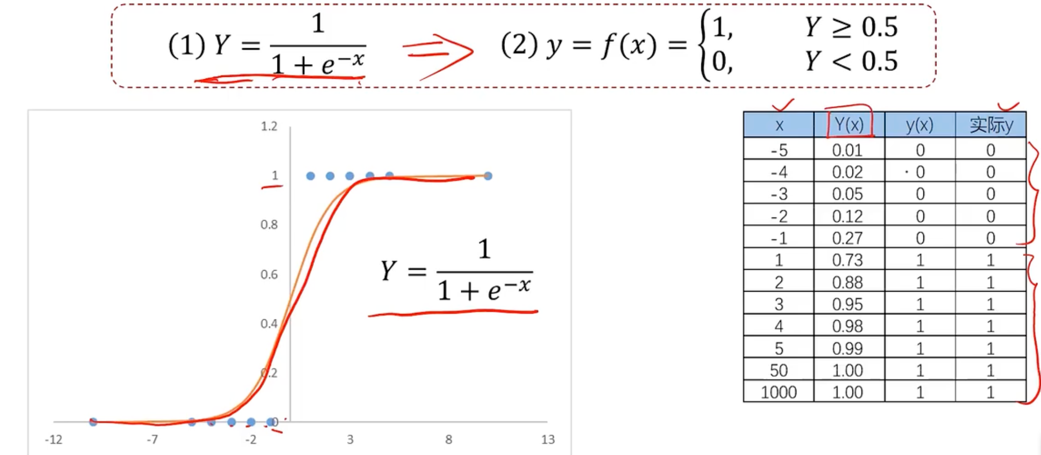
使用逻辑回归拟合数据，可以很好的完成分类问题。思想和线性回归基本一致，但是使用的方程不一样，一个使用线性方程，一个使用逻辑方程。

逻辑回归用于解决分类问题的一种模型，根据数据特征或者属性，计算其回归属于某一类别的概率 $P(x)$ ，根据概率数值判断其所属类型，主要应用于：二分类问题。sigmoid方程如下

$P(x) = \frac{1}{1 + e^{-x}} ,(sigmoid)$

$y=\left\{\begin{matrix}1, P(x)\geqslant 0.5 \\ 0.5, P(x)< 0.5 \end{matrix}\right.$

其中，y为类别结果，P为概率分布哈数，x为特征值。

既然要使用逻辑回归解决或者说替代线性回归，自然是逻辑回归比线性回归有更强的分类能力，试用场景更广。

比如通过x1和x2去判断y的情况如下所示

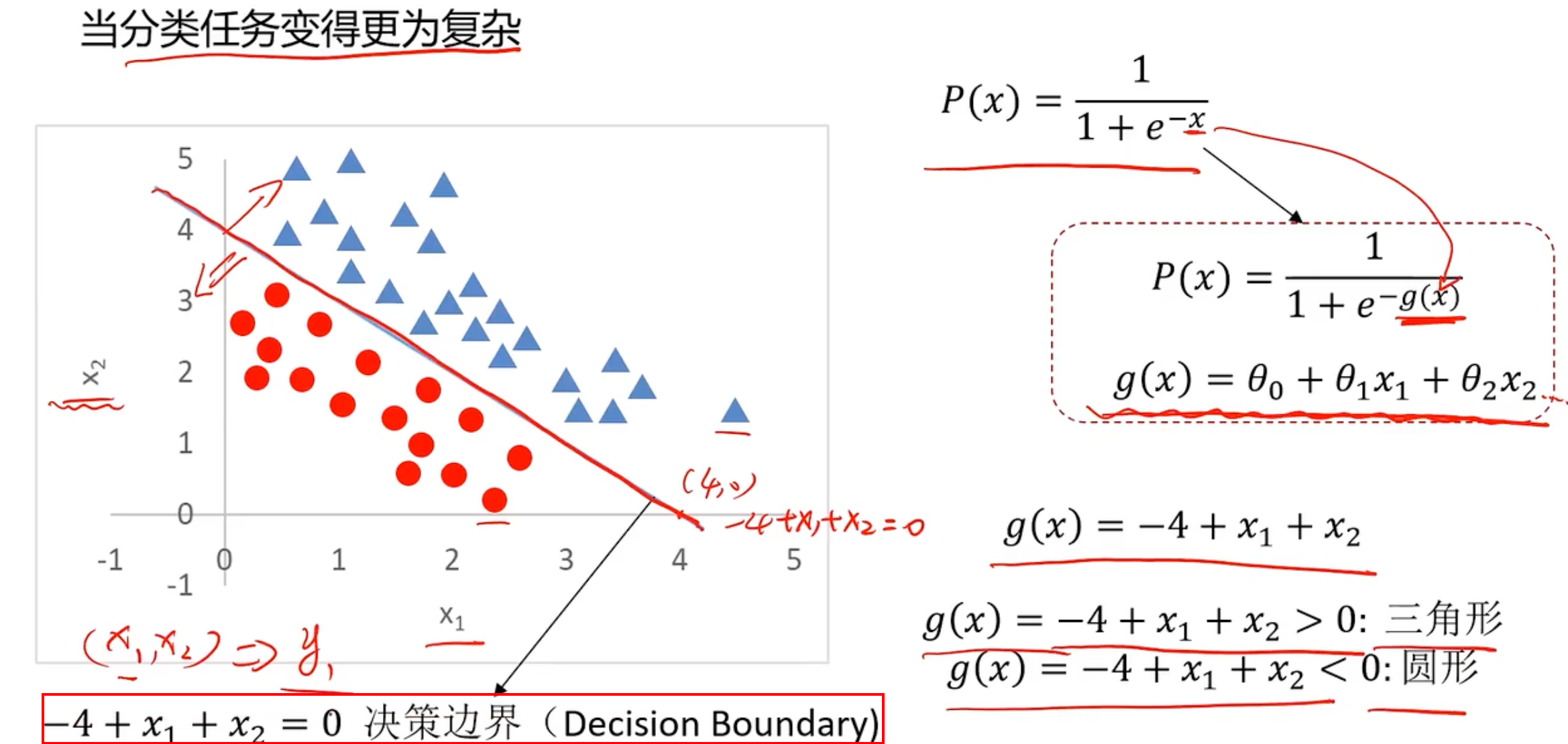
现在的问题就变成了寻找这个这条分界线，即寻找边界函数，或者说寻找g(x)。这个是线性问题，现在有个更复杂的问题，比如

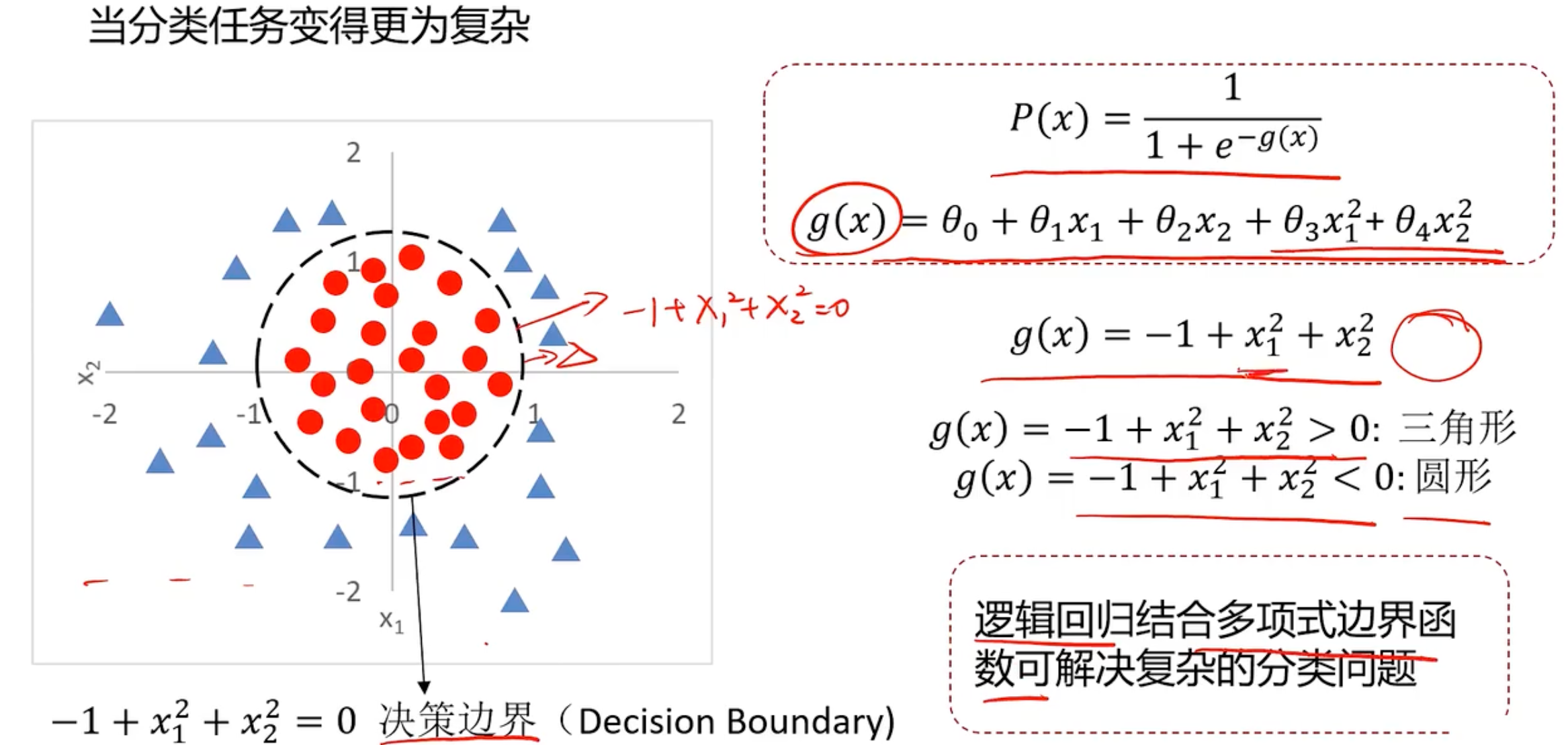
这样就是逻辑回归是很多分类问题的基础。

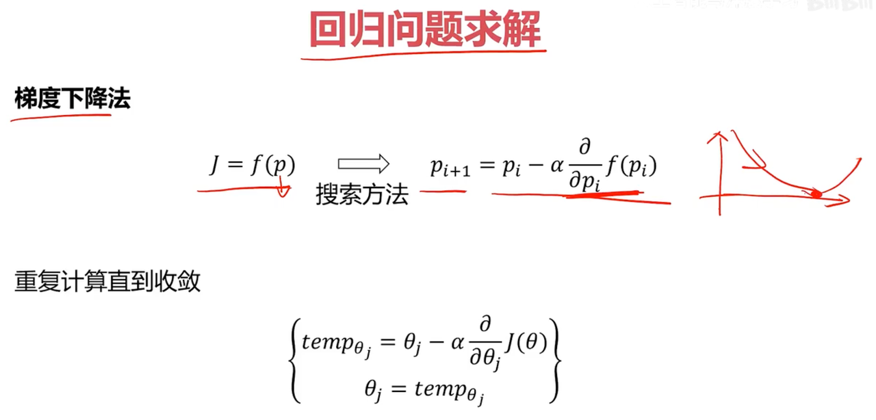
逻辑回归求解，就是寻找边界函数

$P(x) = \frac{1}{1 + e^{-x}} ,(sigmoid)$

$g(x)=\theta _0 +\theta _1x_1+...$

根据训练样本，去寻找 $\theta _0, \theta _1,\theta _2...$

我们知道线性回归求解，就是最小化损失函数 $J$

$J=\frac{1}{2m}\sum_{i=1}^{m}(y_{i}^{'}-y_i)^2$

但是分类问题中，标签和预测结果都是离散点，使用该损失函数无法找到极值点，因为离散的无法求导。那我就定义逻辑回归中，最小化损失函数 $J$

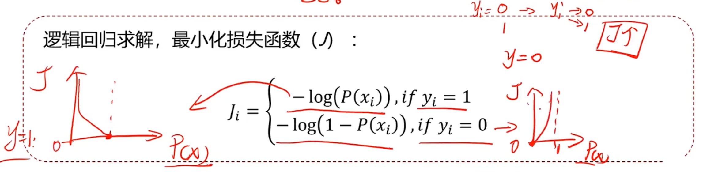
所以逻辑回归求解，最小化损失函数如下所示：

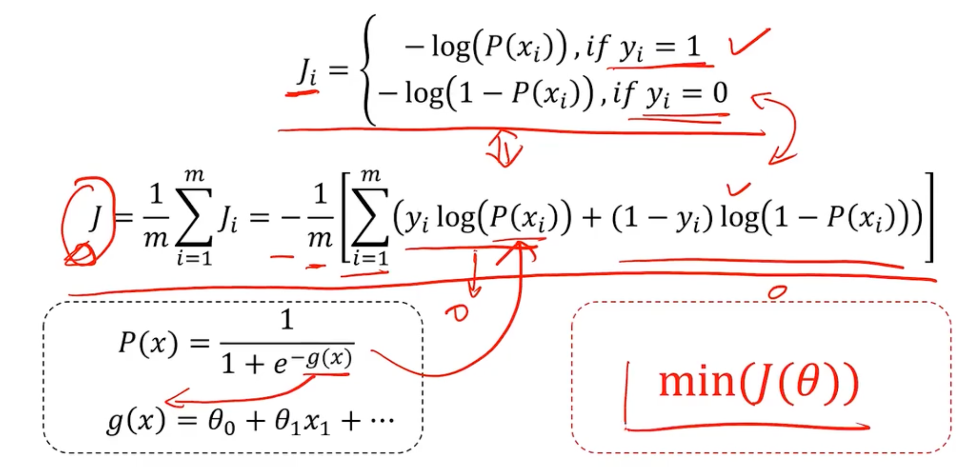
所以整体的求解思想和线性回归是一致的。

现在回过头来再看看为什么叫逻辑回归

名称的由来

数学基础：逻辑回归使用的是逻辑函数（也称为sigmoid函数），该函数能够将输入值映射到0到1之间的一个概率值。这种输出形式非常适合用来表示一个样本属于某个类别的概率。

历史背景：逻辑回归的名字来源于早期统计学中的线性回归模型。尽管它用于分类，但其基本原理与回归分析有相似之处——都是基于对自变量和因变量之间关系的建模。只不过，逻辑回归通过logit变换将线性组合的结果转换为了概率。

为什么叫“回归”

线性模型的基础：逻辑回归本质上是在线性回归的基础上发展而来的，它假设输入特征的线性组合经过一个非线性的激活函数（如sigmoid函数）后可以预测类别概率。因此，从技术角度看，它保留了“回归”的概念，即试图找到自变量与因变量之间的关系。

目标函数的形式：在训练过程中，逻辑回归尝试最小化损失函数（通常是负对数似然），这与线性回归中最小化平方误差的目标函数形式有所不同，但在优化参数的方法上有很多相似之处。

逻辑回归实战准备

分类散点图可视化
逻辑回归模型使用
建立新数据集
模型评估

上述线性函数的在x=0的得到的theta_0称为截距/偏移量/偏执。

那如何生成新的属性数据呢，就是生成 $x_{1}^{2},x_{2}^{2}$

接下来就评估下模型表现.

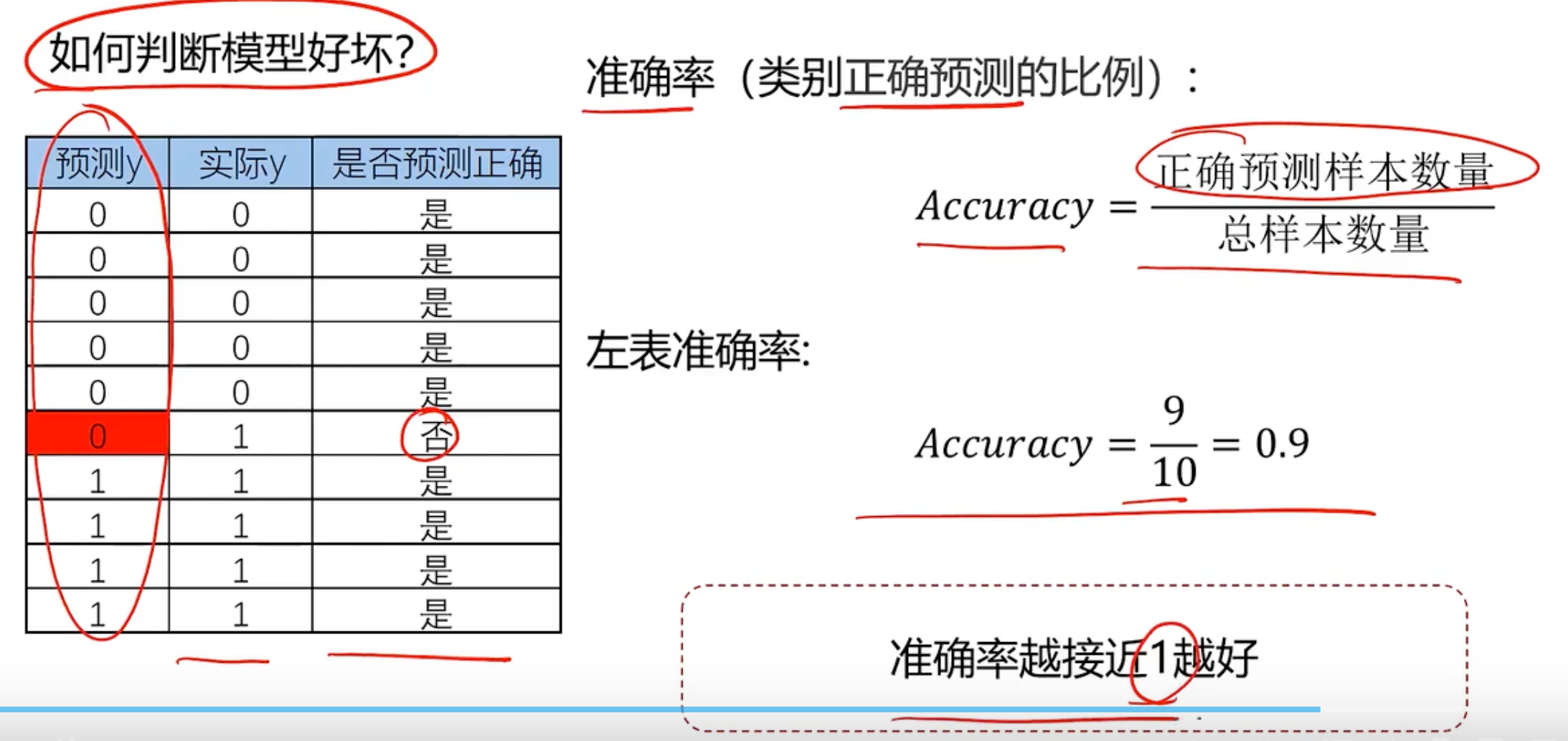
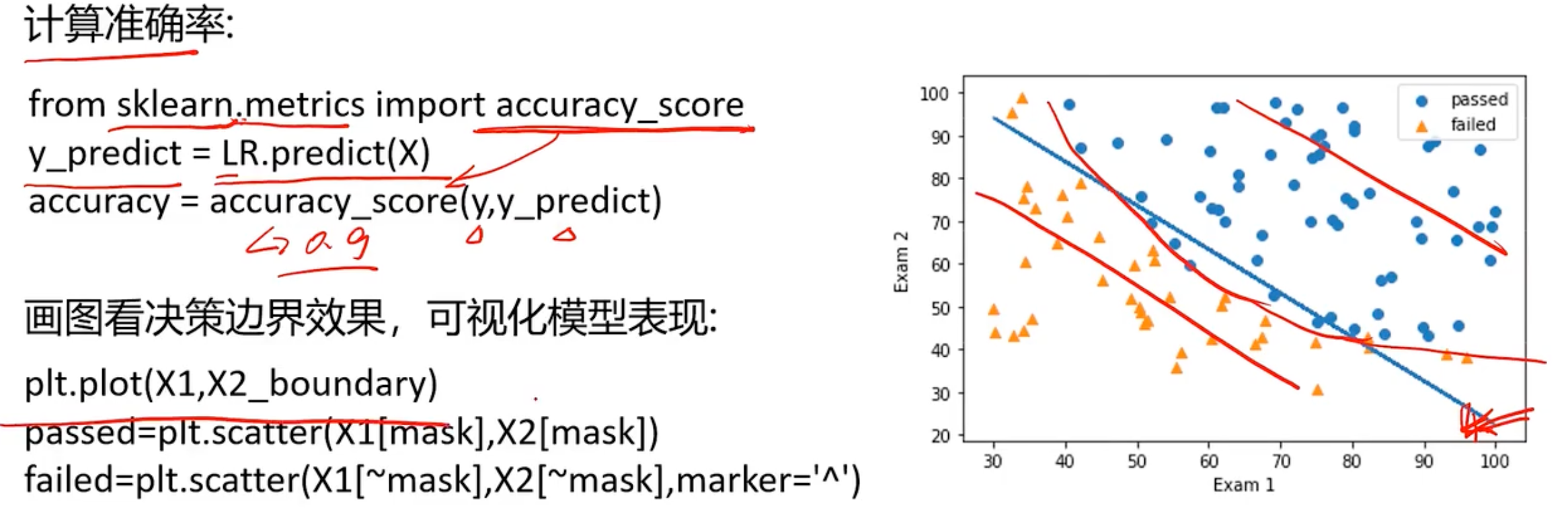
如何计算准确率呢

逻辑回归分类-考试通过预测

一阶线性模型

任务：基于exacmdata.csv数据，建立逻辑回归模型，预测Exam1=75 Exam2=60时，该同学在Exam3试passed or failed

step1 加载数据

import numpy as np
import pandas as pd

from contants import PATH

data = pd.read_csv(PATH + 'examdata.csv')
print(data.head())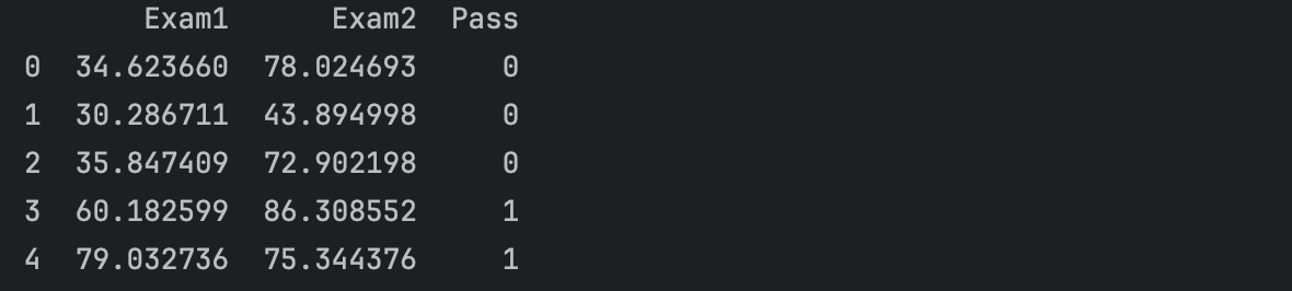

step2 可视化数据

# 可视化我们的数据 visualize the data
from matplotlib import pyplot as plt

fig1 = plt.figure()
#  使用panda的DataFrame，使用.loc函数选取所有的行(:表示所有的行)，选择一个名为"Exam1"的那一列
plt.scatter(data.loc[:, "Exam1"], data.loc[:, "Exam2"])
plt.title("Exam1 - Exam2")
plt.xlabel("Exam1")
plt.ylabel("Exam2")
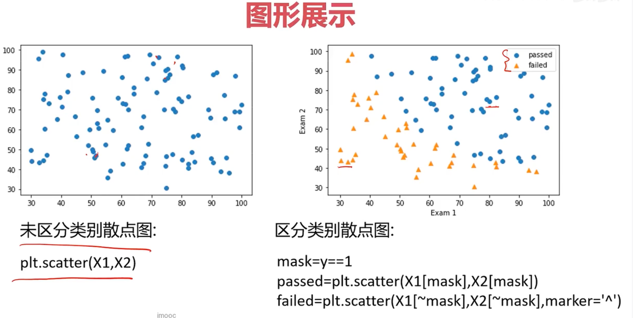
plt.show()

我们加上mask识别通过和没有通过考试的分布

# 上面的是一个散点图，无法区分exam1和exam2的数据，所以需要将不同的数据区分下
# add the mask
mask = data.loc[:, 'Pass'] == 1
print(mask)  # 如果想取反，就print(~mask)
fig2 = plt.figure()
#  使用panda的DataFrame，使用.loc函数选取所有的行(:表示所有的行)，选择一个名为"Exam1"的那一列
passed = plt.scatter(data.loc[:, "Exam1"][mask], data.loc[:, "Exam2"][mask])
failed = plt.scatter(data.loc[:, "Exam1"][~mask], data.loc[:, "Exam2"][~mask])

plt.title("Exam1 - Exam2")
plt.xlabel("Exam1")
plt.ylabel("Exam2")
plt.legend((passed, failed), ('passed', 'failed'))
plt.show()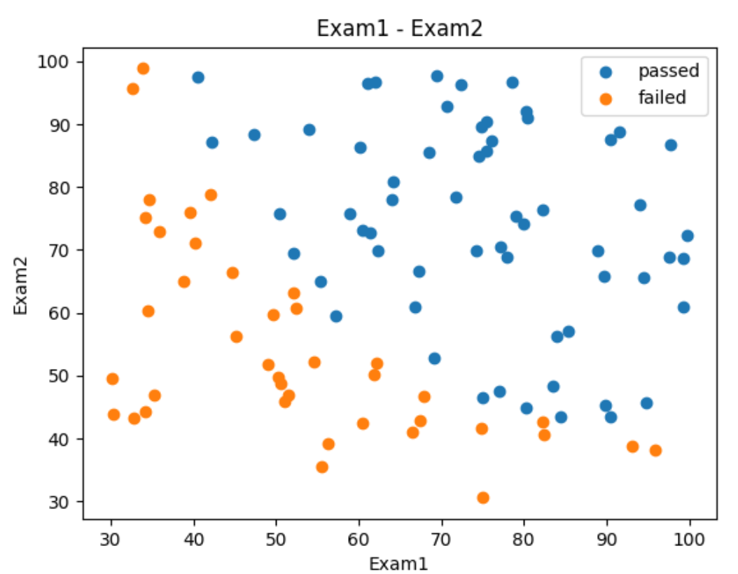

这样就非常明显了，发现成绩在右上角的就是不错的

step3 准备数据

# define X，y数据
X = data.drop(['Pass'], axis=1)
# 上面发现x没有排序后，大小随机会导致绘制图像很混乱，在绘制二阶函数的时候很混乱,可以注释下面这一行
X1 = X1.sort_values()

print(f'输出X的Head信息\n', X.head())
y = data.loc[:, 'Pass']
X1 = data.loc[:, 'Exam1']
X2 = data.loc[:, 'Exam2']
print(X1.head())
print(X2.head())
print(f'输出自变量和因变量的维度: ', X.shape, y.shape)

step4 训练数据

# 一阶线性拟合
# establish the model and train it
from sklearn.linear_model import LogisticRegression
LR = LogisticRegression()
LR.fit(X, y)

# 检查下预测结果
# show the predicted result and its accuracy
y_predict = LR.predict(X)
print(y_predict)

from sklearn.metrics import accuracy_score
accuracy = accuracy_score(y, y_predict)
print("预测评估准确率： ", accuracy)

# 预测下75和60分的同学能否通过考试
# exam1=70, exam2=60
y_test = LR.predict([[70,65]])
print(y_test)
print('passed' if y_test == 1 else 'failed')

输出结果如下所示：

Name: Exam2, dtype: float64
输出自变量和因变量的维度: (100, 2) (100,)
[0 0 0 1 1 0 1 0 1 1 1 0 1 1 0 1 0 0 1 1 0 1 0 0 1 1 1 1 0 0 1 1 0 0 0 0 1
1 0 0 1 0 1 1 0 0 1 1 1 1 1 1 1 0 0 0 1 1 1 1 1 0 0 0 0 0 1 0 1 1 0 1 1 1
1 1 1 1 0 1 1 1 1 0 1 1 0 1 1 0 1 1 0 1 1 1 1 1 0 1]
预测评估准确率： 0.89
[1]
passed

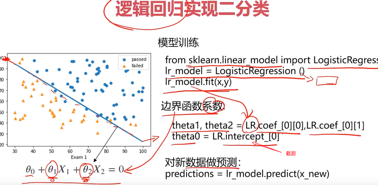
对应的一阶线性模型的边界曲线，我们需要获取截距、斜率等参数。边界函数为

$\theta_0 + \theta_1x_1+\theta_2x_2=0$

theta0 = LR.intercept_
theta1, theta2 = LR.coef_[0][0], LR.coef_[0][1]
print(f"输出模型的三个参数：", theta0, theta1, theta2)

这里的为什么 $\theta_1, \theta_2$ 为什么是上面的求解方式呢？

因为线性回归方程中，有两个输入特征 $x_1,x_2$ 对应的模型就是上述的边界函数， $\theta_1, \theta_2$ 称之为每个特征的权重， $\theta_0$ 为截距。

当使用sklearn.linear_model.LinearRegression做线性回归时，有两个关键属性：

conef_:权重(系数)

intercept_:截距

那为什么LR.conf_是一个二维数组呢？

如果构造的数据是这样的：
X = [[x1_1, x2_1],
     [x1_2, x2_2],
     ...
     [x1_n, x2_n]]
也就是这个是个多样本，每个样本有两个特征，那么
LR = LinearRegression().fit(X, y)
这时LR.conf_是一个二位数组，形状为(1, n_features)，即(1,2)

例如：
LR.coef_ = [[2.5, 3.7]]
所以
LR.coef_[0][0]  # 第一个特征的系数 theta1 = 2.5
LR.coef_[0][1]  # 第二个特征的系数 theta2 = 3.7
为什么是conf[0][i]而不是coef_[i]呢

因为 coef_ 的结构是二维的：(n_targets, n_features)，而你只有一个目标变量 y，所以 n_targets = 1，所以你要用 coef_[0][i] 来取出第 0 个目标的第 i 个特征的系数。

# 接着如何获取这个边界曲线
# 边界函数是theta0 + theta1 * x_1 + theta2 * x_2 = 0
X2_new = -(theta0 + theta1 * X1)/theta2
print(f"X2_new: ", X2_new)
fig3 = plt.figure()
plt.plot(X1, X2_new)
plt.show()

现在我们所有的数据绘制同一个图中

# 现在我们将上面的边界函数和散点数据绘制在一张图片中
fig3 = plt.figure()
passed=plt.scatter(data.loc[:, "Exam1"][mask], data.loc[:, "Exam2"][mask])
failed=plt.scatter(data.loc[:, "Exam1"][~mask], data.loc[:, "Exam2"][~mask])

plt.title("Exam1 - Exam2")
plt.xlabel("Exam1")
plt.ylabel("Exam2")
plt.legend((passed,failed), ('passed', 'failed'))
plt.plot(X1, X2_new)
plt.show()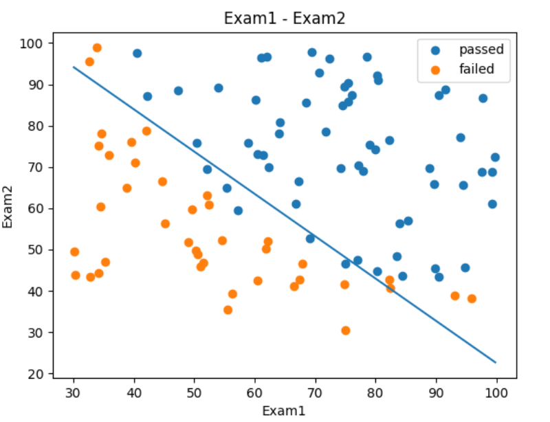

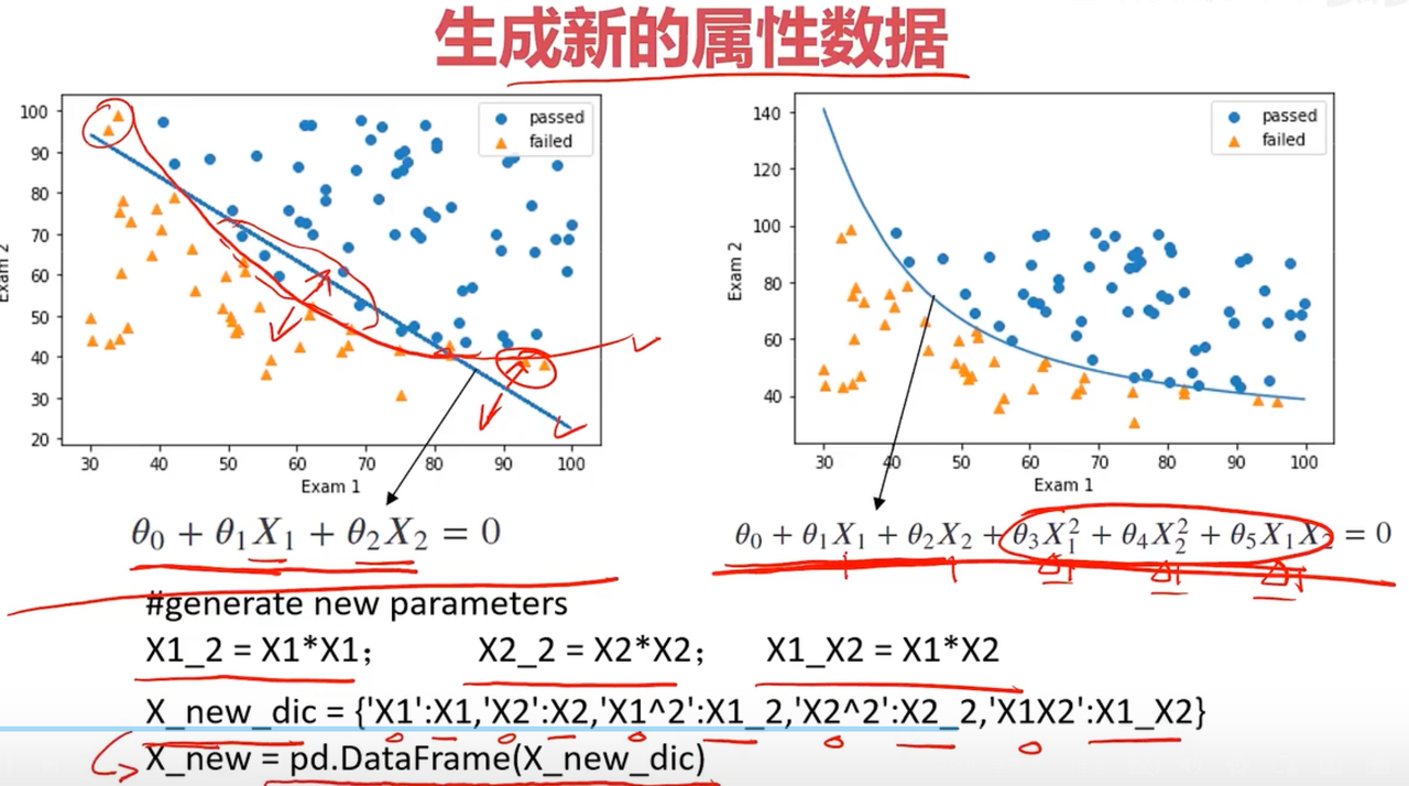
二阶多项式模型实战1

# 创建二阶边界函数， X1和X2的平方
X1_2 = X1 * X1
X2_2 = X2 * X2
X1_X2 = X1 * X2
print('输出x_1和x1_2: ', X1, X1_2)
X_new = {'X1': X1, 'X2': X2, 'X1_2': X1_2, 'X2_2': X2_2, 'X1_X2': X1_X2}
X_new = pd.DataFrame(X_new)
print(X_new)

输出x_1和x1_2: 63 30.058822
1 30.286711
57 32.577200
70 32.722833
36 33.915500
...

# establish new model and train
from sklearn.metrics import accuracy_score

# LR2 = LogisticRegression()
LR2 = LogisticRegression(solver='lbfgs', max_iter=1000)
LR2.fit(X_new, y)
y2_predict = LR2.predict(X_new)
accuracy2 = accuracy_score(y, y2_predict)
print('二阶模型准确率: ',accuracy2)

二阶模型准确率: 1.0

求解边界函数

现在在训练函集中， $X_*$ 是已知的，求解各个 $\theta_*$ 参数。

print("coef_: ",LR2.coef_)

coef_: [[ 0.00217087 -0.00065115 -0.02025598 -0.01999855 0.17601132]]

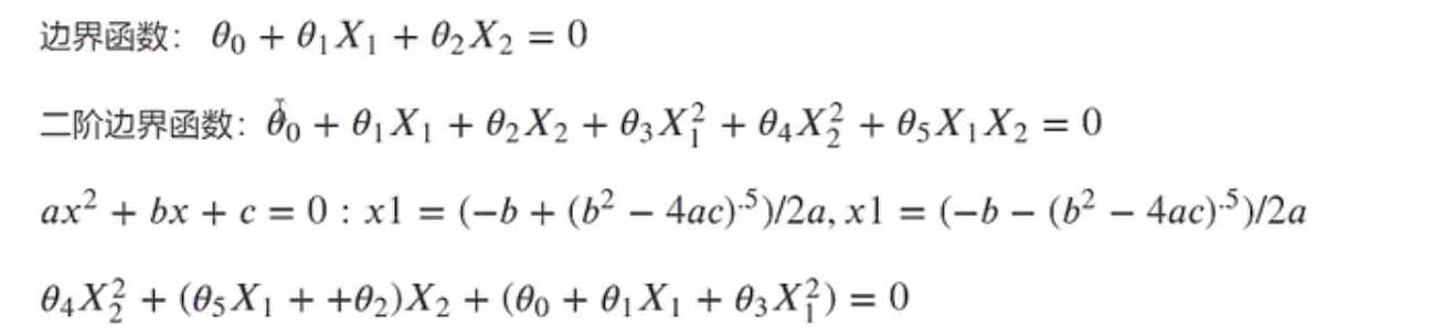
绘制二阶边界曲线

# 更直观的看，我们画出来
theta0 = LR2.intercept_
theta1, theta2, theta3, theta4, theta5 = LR2.coef_[0][0], LR2.coef_[0][1], LR2.coef_[0][2], LR2.coef_[0][3], \
LR2.coef_[0][4]
a = theta4
b = theta5 * X1 + theta2
c = theta0 + theta1 * X1 + theta3 * X1 * X1
print(theta0, theta1, theta2, theta3, theta4, theta5)

X2_new_boundary = (-b + np.sqrt(b * b - 4 * a * c)) / (2 * a)
print(X2_new_boundary)

fig4 = plt.figure()
plt.plot(X1, X2_new_boundary)
plt.show()

这里求解二阶系数为什么不取负的呢，即

(-b - np.sqrt(b * b - 4 * a * c)) / (2 * a)

因为成绩是正数

#  绘制在一起
fig5 = plt.figure()
passed = plt.scatter(data.loc[:, "Exam1"][mask], data.loc[:, "Exam2"][mask])
failed = plt.scatter(data.loc[:, "Exam1"][~mask], data.loc[:, "Exam2"][~mask])

plt.title("Exam1 - Exam2")
plt.xlabel("Exam1")
plt.ylabel("Exam2")
plt.legend((passed, failed), ('passed', 'failed'))
plt.plot(X1, X2_new_boundary)
plt.show()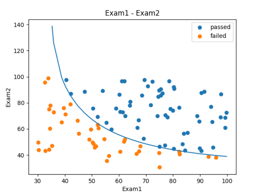

如果是三阶函数，四阶函数可能准确率会有所提升。

有了上面的经验，建立逻辑回归模型有了一定基础，这里再给出一个示例

二阶多项式模型实战2

step1加载数据

from matplotlib import pyplot as plt
from sklearn.linear_model import LogisticRegression
import numpy as np
import pandas as pd

from contants import PATH

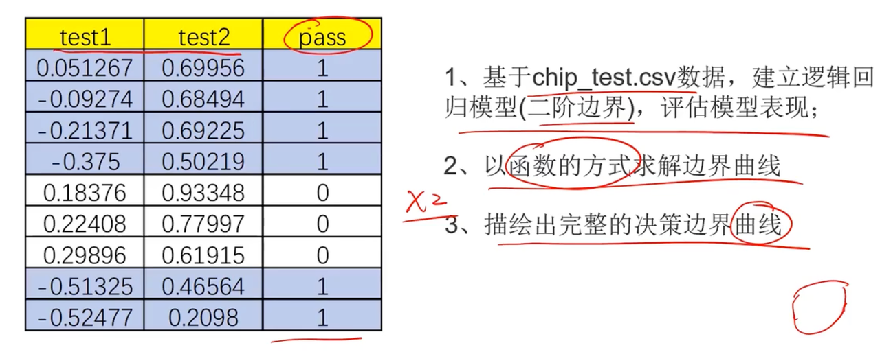
data = pd.read_csv(PATH + 'chip_test.csv')
print(data.head())

step2可视化数据

# 可视化
fig1 = plt.figure()
passed=plt.scatter(data.loc[:, "test1"][mask], data.loc[:, "test2"][mask])
failed=plt.scatter(data.loc[:, "test1"][~mask], data.loc[:, "test2"][~mask])

plt.title("test1 - test2")
plt.xlabel("test1")
plt.ylabel("test2")
plt.legend((passed,failed), ('passed', 'failed'))
plt.show()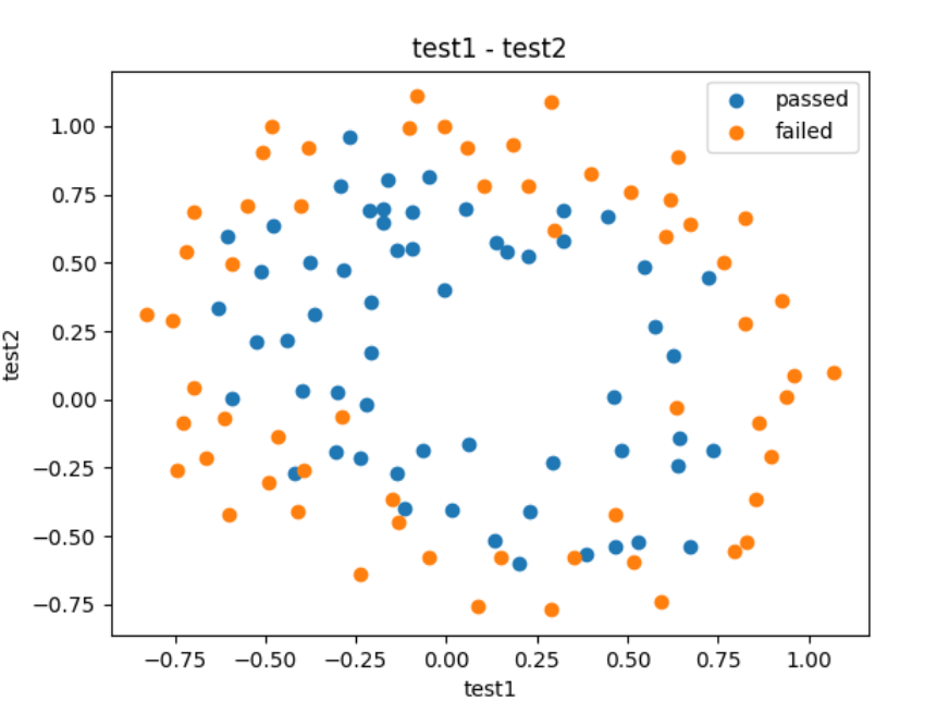

发现上述的数据一阶肯定是无法拟合的，只能通过多阶多项式的方式进行拟合

step3准备数据

# # generate new data,进入二阶数据拟合
# define X，y数据
X = data.drop(['pass'], axis=1)

print(f'输出X的Head信息\n', X.head())
y = data.loc[:, 'pass']
X1 = data.loc[:, 'test1']

# establish model and train it;predit
from sklearn.metrics import accuracy_score

LR2 = LogisticRegression()
# LR2 = LogisticRegression(solver='lbfgs', max_iter=1000)
LR2.fit(X_new, y)

# accuracy
y2_predict = LR2.predict(X_new)
accuracy2 = accuracy_score(y, y2_predict)
print(f'数据预测: ', accuracy2)

绘制输出内容

# # decision boundary
# 更直观的看，我们画出来
X1_new = X1.sort_values()
theta0 = LR2.intercept_
theta1, theta2, theta3, theta4, theta5 = LR2.coef_[0][0], LR2.coef_[0][1], LR2.coef_[0][2], LR2.coef_[0][3], \
LR2.coef_[0][4]
a = theta4
b = theta5 * X1_new + theta2
c = theta0 + theta1 * X1_new + theta3 * X1_new * X1_new
print(theta0, theta1, theta2, theta3, theta4, theta5)
X2_new_boundary = (-b + np.sqrt(b*b-4*a*c))/(2*a)
# #  绘制在一起
fig2 = plt.figure()
passed=plt.scatter(data.loc[:, "test1"][mask], data.loc[:, "test2"][mask])
failed=plt.scatter(data.loc[:, "test1"][~mask], data.loc[:, "test2"][~mask])
plt.plot(X1_new, X2_new_boundary)

plt.title("test1 - test2")
plt.xlabel("test1")
plt.ylabel("test2")
plt.legend((passed,failed), ('passed', 'failed'))
plt.show()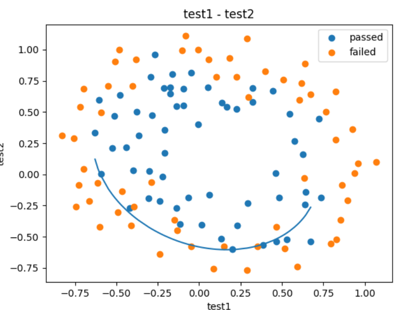

为什么只有一半呢，因为上文中提到了我们没有取

(-b - np.sqrt(b * b - 4 * a * c)) / (2 * a

step4训练数据

定义函数的方式求解

# define f(X)
def f(x):
    a = theta4
    b = theta5 * x + theta2
    c = theta0 + theta1 * x + theta3 * x * x
    print(theta0, theta1, theta2, theta3, theta4, theta5)

    X2_new_boundary1 = (-b + np.sqrt(b * b - 4 * a * c)) / (2 * a)
    X2_new_boundary2 = (-b - np.sqrt(b * b - 4 * a * c)) / (2 * a)
    return X2_new_boundary1, X2_new_boundary2

X2_new_boundary1  = []
X2_new_boundary2 = []

for x in X1_new:
    X2_new_boundary1.append(f(x)[0])
    X2_new_boundary2.append(f(x)[1])
print(X2_new_boundary1, X2_new_boundary2)

fig3 = plt.figure()
passed=plt.scatter(data.loc[:, "test1"][mask], data.loc[:, "test2"][mask])
failed=plt.scatter(data.loc[:, "test1"][~mask], data.loc[:, "test2"][~mask])

plt.title("test1 - test2")
plt.xlabel("test1")
plt.ylabel("test2")
plt.legend((passed,failed), ('passed', 'failed'))
plt.plot(X1_new, X2_new_boundary1)
plt.plot(X1_new, X2_new_boundary2)
plt.show()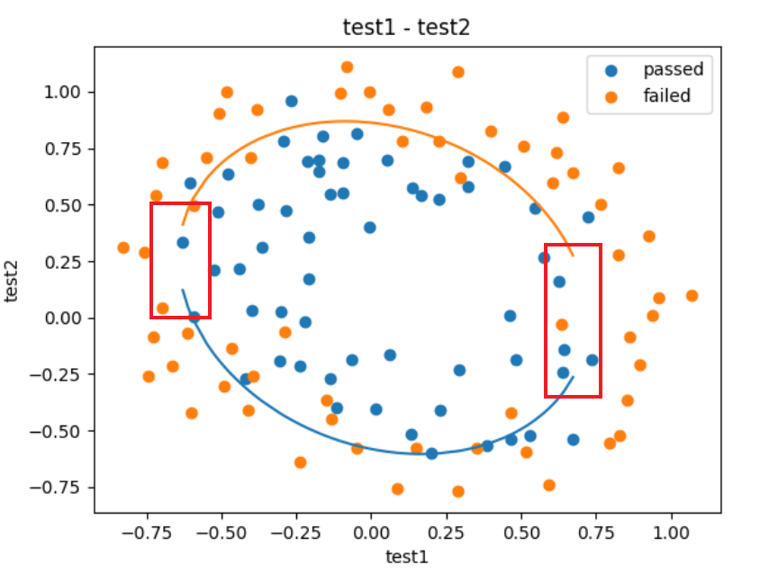

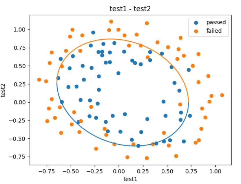
发现少了一块，因为参数中是离散的，有间隔的所以导致最后的数据展示“不全”，现在我们需要把它补上

# 补充并创建数据集
X1_range = [-0.9 + x/10000 for x in range(0, 20000)]
X1_range = np.array(X1_range)
X2_new_boundary1 = []
X2_new_boundary2 = []
for x in X1_range:
    X2_new_boundary1.append(f(x)[0])
    X2_new_boundary2.append(f(x)[1])

fig3 = plt.figure()
passed=plt.scatter(data.loc[:, "test1"][mask], data.loc[:, "test2"][mask])
failed=plt.scatter(data.loc[:, "test1"][~mask], data.loc[:, "test2"][~mask])
plt.title("test1 - test2")
plt.xlabel("test1")
plt.ylabel("test2")
plt.legend((passed,failed), ('passed', 'failed'))
plt.plot(X1_range, X2_new_boundary1)
plt.plot(X1_range, X2_new_boundary2)
plt.show()

分类问题之逻辑回归

什么是逻辑回归

逻辑回归实战准备

逻辑回归分类-考试通过预测

一阶线性模型

step1 加载数据

step2 可视化数据

step3 准备数据

step4 训练数据

二阶多项式模型实战1

二阶多项式模型实战2

step1加载数据

step2可视化数据

step3准备数据

step4训练数据

网站公告

今日签到

热门文章

最新发布