目录
1 构建分类器
为MNIST数据集构建一个分类器,并在测试集上达成超过97%的精度。
下面进行代码展示:
#1、获取MNIST数据集
from sklearn.datasets import fetch_openml
mnist = fetch_openml('mnist_784', version=1, cache=True, as_frame=False)

#2、划分数据集
import numpy as np

X, y = mnist["data"], mnist["target"]

#MNIST默认划分的训练集和测试集
X_train, X_test, y_train, y_test = X[:60000], X[60000:], y[:60000], y[60000:]

#数据重新洗牌,防止算法对训练实例的顺序敏感
shuffle_index = np.random.permutation(60000)#生成一个随机排列的数组
X_train, y_train = X_train[shuffle_index], y_train[shuffle_index]


#注意对自己电脑硬件不自信不要运行下面代码,以防蓝屏,可以了解一下思想
from sklearn.neighbors import KNeighborsClassifier
from sklearn.model_selection import GridSearchCV

param_grid = [{'weights': ["uniform", "distance"], 'n_neighbors': [3, 4, 5]}]

knn_clf = KNeighborsClassifier()
grid_search = GridSearchCV(knn_clf, param_grid, cv=5, verbose=3, n_jobs=-1)
grid_search.fit(X_train, y_train)
找到合适的超参数:
grid_search.best_params_运行结果如下:
{'n_neighbors': 4, 'weights': 'distance'}得分:
grid_search.best_score_运行结果如下:
0.97325预测精度:
from sklearn.metrics import accuracy_score

y_pred = grid_search.predict(X_test)
accuracy_score(y_test, y_pred)
运行结果如下:
0.9714我们就代码中包含的知识点进行简单讲解:
1.1 np.random.permutation()
对给定的数组重新排列。
import numpy as np

arr = np.random.permutation(6)
print(arr)
运行结果如下:
[2 5 4 0 3 1]另外对数组进行重新排列的还包括:np.random.shuffle(arr)
arr = np.arange(6)
print(arr)
np.random.shuffle(arr)
print(arr)
运行结果如下:
[0 1 2 3 4 5]
[4 5 1 2 0 3]
1.2 KNeighborsClassifier()
中文文档说明:sklearn.neighbors.KNeighborsClassifier-scikit-learn中文社区
英文文档说明:sklearn.neighbors.KNeighborsClassifier — scikit-learn 1.1.2 documentation
我们看一下文档中参数:
sklearn.neighbors.KNeighborsClassifier(n_neighbors=5, *, weights='uniform', algorithm='auto', leaf_size=30, p=2, metric='minkowski', metric_params=None, n_jobs=None, **kwargs)| 参数 | 说明 |
|---|---|
| n_neighbors | int, default=5 默认情况下用于kneighbors查询的近邻数 |
| weights | {‘uniform’, ‘distance’} or callable, default=’uniform’ 预测中使用的权重函数。 可能的值: “uniform”:统一权重。 每个邻域中的所有点均被加权。 “distance”:权重点与其距离的倒数。 在这种情况下,查询点的近邻比远处的近邻具有更大的影响力。 [callable]:用户定义的函数,该函数接受距离数组,并返回包含权重的相同形状的数组。 |
| algorithm | {‘auto’, ‘ball_tree’, ‘kd_tree’, ‘brute’}, default=’auto’ 用于计算最近临近点的算法: “ ball_tree”将使用BallTree kd_tree”将使用KDTree “brute”将使用暴力搜索。 “auto”将尝试根据传递给fit方法的值来决定最合适的算法。 注意:在稀疏输入上进行拟合将使用蛮力覆盖此参数的设置。 |
| leaf_size | int, default=30 叶大小传递给BallTree或KDTree。 这会影响构造和查询的速度,以及存储树所需的内存。 最佳值取决于问题的性质。 |
| p | int, default=2 Minkowski指标的功率参数。 当p = 1时,这等效于对p = 2使用manhattan_distance(l1)和euclidean_distance(l2)。对于任意p,使用minkowski_distance(l_p)。 |
| metric | str or callable, default=’minkowski’ 树使用的距离度量。 默认度量标准为minkowski,p = 2等于标准欧几里德度量标准。 有关可用度量的列表,请参见DistanceMetric的文档。 如果度量是“预先计算的”,则X被假定为距离矩阵,并且在拟合过程中必须为平方。 X可能是一个稀疏图,在这种情况下,只有“非零”元素可以被视为临近点。 |
| metric_params | dict, default=None 度量功能的其他关键字参数。 |
| n_jobs | int, default=None 为临近点搜索运行的并行作业数。 除非在joblib.parallel_backend上下文中,否则None表示1。 -1表示使用所有处理器。 有关更多详细信息,请参见词汇表。 不会影响拟合方法。 |
我们再看一下属性:
| 属性 | 说明 |
|---|---|
| classes_ | array of shape (n_classes,) 分类器已知的类标签 |
| effective_metric_ | str or callble 使用的距离度量。 它将与度量参数相同或与其相同,例如 如果metric参数设置为“ minkowski”,而p参数设置为2,则为“ euclidean”。 |
| effective_metric_params_ | dict 度量功能的其他关键字参数。 对于大多数指标而言,它与metric_params参数相同,但是,如果将valid_metric_属性设置为“ minkowski”,则也可能包含p参数值。 |
| outputs_2d_ | bool 在拟合期间,当y的形状为(n_samples,)或(n_samples,1)时为False,否则为True。 |
方法:
| 方法 | 说明 |
|---|---|
fit(, X, y) |
使用X作为训练数据和y作为目标值拟合模型 |
get_params([, deep]) |
获取此估计量的参数。 |
kneighbors([, X, n_neighbors, …]) |
查找点的K临近点。 |
kneighbors_graph([, X, n_neighbors, mode]) |
计算X中点的k临近点的(加权)图 |
predict(, X) |
预测提供的数据的类标签。 |
predict_proba(, X) |
测试数据X的返回概率估计。 |
score(, X, y[, sample_weight]) |
返回给定测试数据和标签上的平均准确度。 |
set_params(, **params) |
设置此估算器的参数。 |
1.3 GridSearchCV()
中文文档说明:sklearn.model_selection.GridSearchCV-scikit-learn中文社区
英文文档说明:sklearn.model_selection.GridSearchCV — scikit-learn 1.1.2 documentation
同样,我们看一下文档中的参数:
sklearn.model_selection.GridSearchCV(estimator, param_grid, *, scoring=None, n_jobs=None, iid='deprecated', refit=True, cv=None, verbose=0, pre_dispatch='2*n_jobs', error_score=nan, return_train_score=False)| 参数 | 说明 |
|---|---|
| estimator | estimator object 假定这样做是为了实现scikit-learn估计器接口。估计器需要提供 score功能,或者必须通过scoring。 |
| param_grid | dict or list of dictionaries 以参数名称( str)作为键,将参数设置列表尝试作为值的字典,或此类字典的列表,在这种情况下,将探索列表中每个字典所跨越的网格。这样可以搜索任何顺序的参数设置。 |
| scoring | str, callable, list/tuple or dict, default=None 单个str(请参阅评分参数:定义模型评估规则)或可调用项(请参阅从度量函数定义评分策略),用于评估测试集上的预测。 要评估多个指标,请给出(唯一的)字符串列表或以名称为键,可调用项为值的字典。 注意,使用自定义评分器时,每个评分器应返回一个值。返回值列表或数组的度量函数可以包装到多个评分器中,每个评分器都返回一个值。 有关示例,请参阅指定多个度量进行评估。 如果为None,则使用估计器的评分方法。 |
| n_jobs | int, default=None 要并行运行的CPU内核数。 None除非在joblib.parallel_backend环境中,否则表示1 。 -1表示使用所有处理器。有关 更多详细信息,请参见词汇表。v0.20版中的更改: n_jobs默认从1更改为None |
| pre_dispatch | int, or str, default=n_jobs 控制在并行执行期间分派的CPU内核数。当调度的CPU内核数量超过CPU的处理能力时,减少此数量可能有助于避免内存消耗激增。该参数可以是: - None,在这种情况下,所有CPU内核都将立即创建并产生,使它进行轻量级和快速运行的任务,以避免因按需生成作业而造成延迟 -int,给出所产生的总CPU内核数的确切数量 -str,根据n_jobs给出表达式,如'2*n_jobs' |
| iid | bool, default=False 如果为True,则按折数返回平均得分,并按每个测试集中的样本数加权。在这种情况下,假定数据在折叠上分布相同,并且最小化的损失是每个样品的总损失,而不是折叠的平均损失。 从版本0.22开始 iid不推荐使用*:*参数在0.22中不再推荐使用,并将在0.24中删除 |
| cv | int, cross-validation generator or an iterable, default=None 确定交叉验证切分策略。可以输入: -None,默认使用5折交叉验证 -integer,用于指定在 (Stratified)KFold中的折叠次数-CV splitter -一个输出训练集和测试集切分为索引数组的迭代。 对于integer或None,如果估计器是分类器,并且 y是二分类或多分类,使用StratifiedKFold。在所有其他情况下,使用KFold。有关可在此处使用的各种交叉验证策略,请参阅用户指南。 在0.22版本中: cv为“None”时,默认值从3折更改为5折 |
| refit | bool, str, or callable, default=True 使用在整个数据集中找到的最优参数重新拟合估计器。 对于多指标评估,这需要是一个表示评分器的 str,该评分器将为最终重新拟合估计器找到最优参数。如果在选择最优估计值时除了考虑最大得分外,还需要考虑其他因素,可以将 refit设置为返回所选best_index_给定cv_results_的函数。在这种情况下,best_estimator_和best_params_将根据返回的best_index_进行设置,而best_score_ 属性将不可用。重新拟合的估计器在 best_estimator_ 属性上可用,并允许predict直接在GridSearchCV实例上使用。同样对于多指标评估, best_index_, best_score_和best_params_属性仅在设置refit时可用,并且都将根据这个特定的评分器来决定。请参阅 scoring参数以了解有关多指标评估的更多信息。在0.20版中:添加了对Callable的支持。 |
| verbose | integer 控制详细程度:越高,消息越多。 |
| error_score | ‘raise’ or numeric, default=np.nan 如果估计器拟合出现错误,将值分配给分数。如果设置为“ raise”,则会引发错误。如果给出数值,则引发FitFailedWarning。此参数不会影响重新拟合步骤,这将总是引发错误。 |
| return_train_score | bool, default=False 如果为 False,则cv_results_属性将不包括训练集分数。计算训练集分数用于了解不同的参数设置如何影响过拟合或欠拟合的权衡。但是,在训练集上计算分数可能在计算上很耗时,并且不严格要求选择产生最优泛化性能的参数。版本0.19中的新功能。 在版本0.21中:默认值将 True更改为False |
属性:
| 属性 | 说明 |
|---|---|
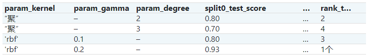
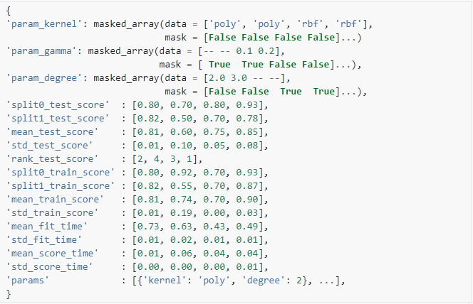
| cv_results_ | dict of numpy (masked) ndarrays 可以将键作为列标题和值作为列的字典导入pandas DataFrame。例如下面给定的表
用一个
注意 |
| best_estimator_ | estimator 搜索选择的估计器,例如,对剩余数据给出最高分(或最小损失是否指定)的估计量。如果设置 refit=False则不可用。有关 refit允许值的更多信息,请参见参数。 |
| best_score_ | float best_estimator的平均交叉验证得分 对于多指标评估,只有在 refit指定时才存在。如果 refit为函数,则此属性不可用。 |
| best_params_ | dict 参数设置可使保留数据获得最优结果。 对于多指标评估,只有在 refit指定时才存在。 |
| best_index_ | search.cv_results_['params'][search.best_index_]的字典给出了最优模型的参数设置,该模型给出最高平均得分(search.best_score_)。对于多指标评估,只有在 refit指定时才存在。 |
| scorer_ | function or a dict 在保留的数据上使用评分器功能为模型选择最优参数。 对于多指标评估,此属性保存已验证的 scoring字典,该字典将评分器键映射到可调用的评分器。 |
| n_splits_ | int 交叉验证切分(或折叠、迭代)的数量。 |
| refit_time_ | float 用于在整个数据集中重新拟合最优模型的秒数。 仅当 refit不是False 时才存在。0.20版中的新功能。 |
方法:
| 方法 | 说明 |
|---|---|
decision_function(self, X) |
使用找到的最优参数在估计器上调用Decision_function。 |
fit(self, X[, y, groups]) |
拟合所有参数组合。 |
get_params(self[, deep]) |
获取此估计器的参数。 |
inverse_transform(self, Xt) |
用找到的最优参数在估计器上调用inverse_transform。 |
predict(self, X) |
使用找到的最优参数在估计器上调用预测。 |
predict_log_proba(self, X) |
使用找到的最优参数在估计器上调用predict_log_proba。 |
predict_proba(self, X) |
使用找到的最优参数在估计器上调用predict_proba。 |
score(self, X[, y]) |
如果估计器已调整,则返回给定数据的分数。 |
set_params(self, **params) |
设置此估计器的参数。 |
transform(self, X) |
使用找到的最优参数在估计器上调用transform。 |
2 数据处理
我们以Titanic数据集为例:
数据下载地址:Titanic - Machine Learning from Disaster | Kaggle
2.1 Kaggle注册
如果不想注册Kaggle再下载,下面网盘直接获取数据:
链接:https://pan.baidu.com/s/1ByllEwkChhk1fKO2mBrbvw
提取码:whj6
如果你坚持下载,但是在注册时出现了“人机验证问题”,解决方法如下:
因为Chrome应用商店是锁着的,下面我就以Edge浏览器为例:


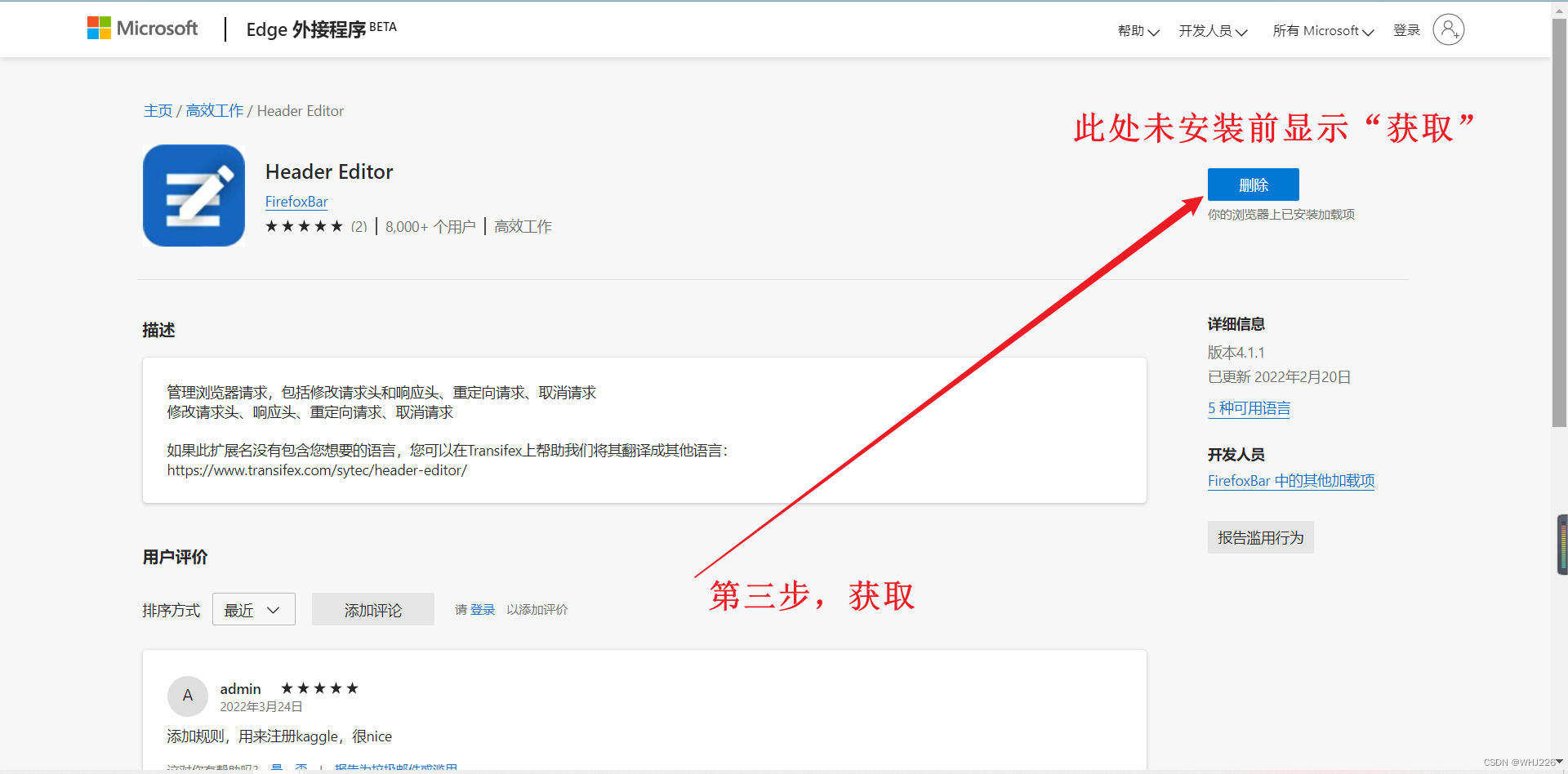


我们输入以下URL:
https://azurezeng.github.io/static/HE-GoogleRedirect.json
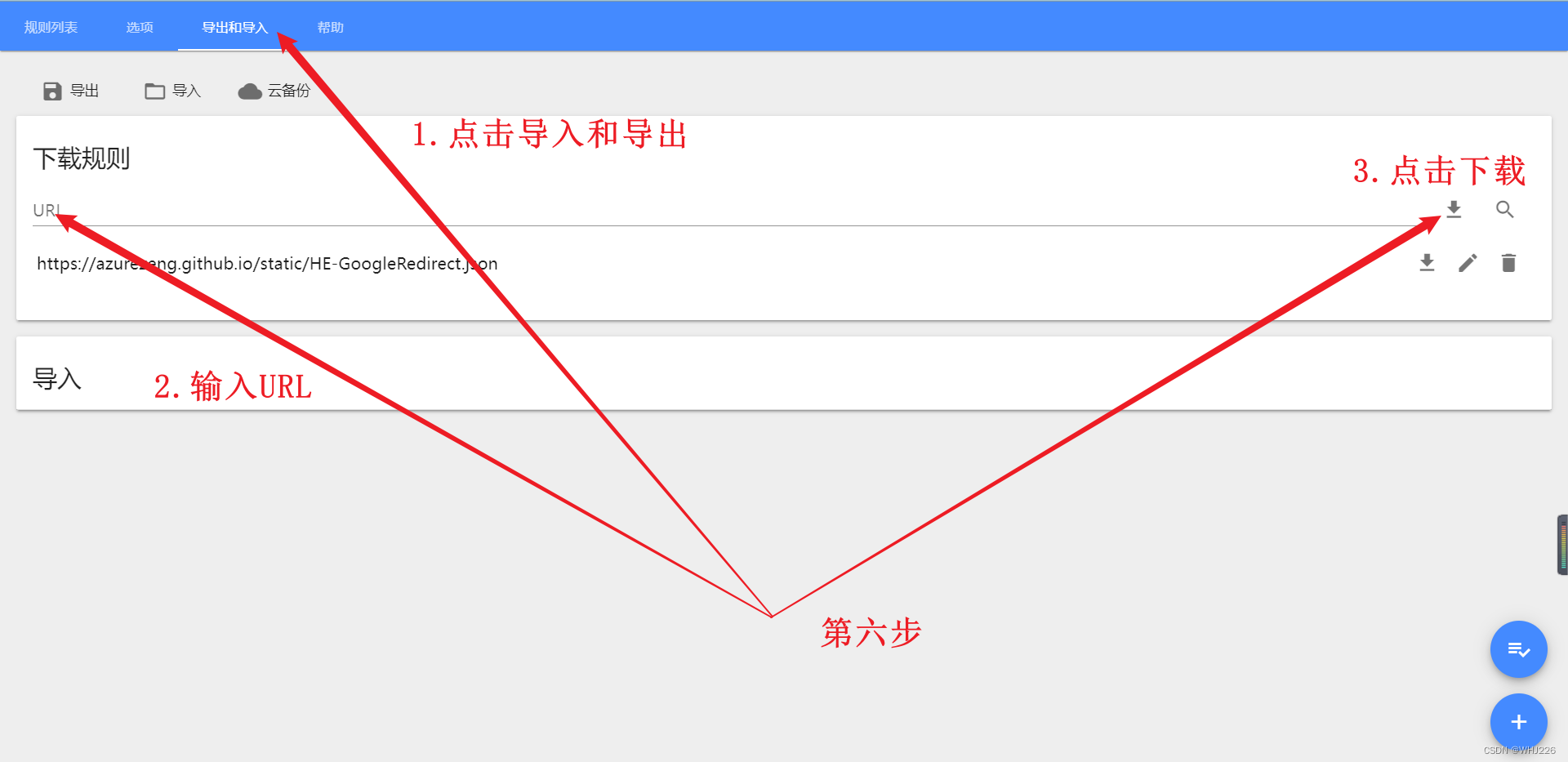
完成后点击保存,重启浏览器即可出现人机验证。
以上内容参考自:Google 人机验证(reCaptcha)无法显示解决方案(可解决大多数 CSP 问题) – Azure Zeng Blog
为了表示感谢,大家可以点击该博文进行阅读!
2.2 Titanic数据处理
首先,我们加载数据:
import pandas as pd

train_data = pd.read_csv("E:/PYTHON/train.csv")
test_data = pd.read_csv("E:/PYTHON/test.csv")
数据已经分为训练集和测试集。但是,测试数据不包含标签:我们的目标是使用训练数据训练出最好的模型,然后根据测试数据进行预测。
我们可以通过head()方法查看训练数据的前5行:
train_data.head()运行结果如下:
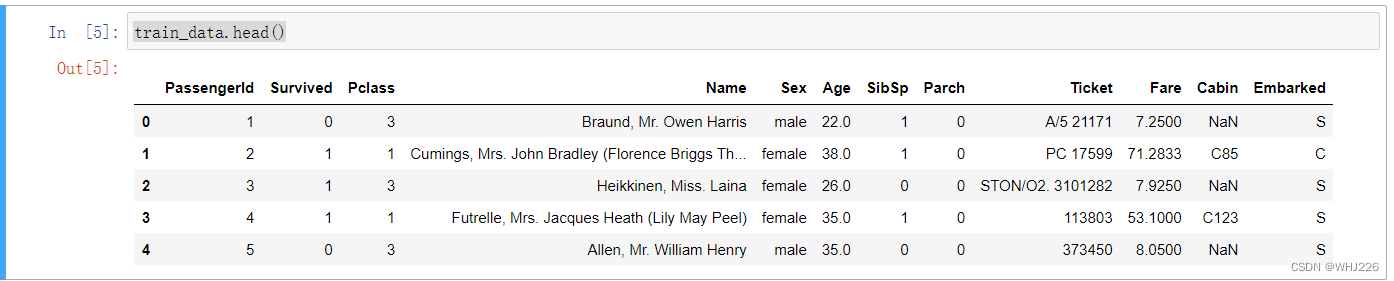
运行结果中的属性有以下含义:
- Survived: that's the target, 0 means the passenger did not survive, while 1 means he/she survived.
- Pclass: passenger class.
- Name, Sex, Age: self-explanatory
- SibSp: how many siblings & spouses of the passenger aboard the Titanic.
- Parch: how many children & parents of the passenger aboard the Titanic.
- Ticket: ticket id
- Fare: price paid (in pounds)
- Cabin: passenger's cabin number
- Embarked: where the passenger embarked the Titanic
由于该数据是有缺失的,我们可以看一下:
train_data.info()运行结果如下:
<class 'pandas.core.frame.DataFrame'>
RangeIndex: 891 entries, 0 to 890
Data columns (total 12 columns):
 #   Column       Non-Null Count  Dtype
---  ------       --------------  -----
 0   PassengerId  891 non-null    int64
 1   Survived     891 non-null    int64
 2   Pclass       891 non-null    int64
 3   Name         891 non-null    object
 4   Sex          891 non-null    object
 5   Age          714 non-null    float64
 6   SibSp        891 non-null    int64
 7   Parch        891 non-null    int64
 8   Ticket       891 non-null    object
 9   Fare         891 non-null    float64
 10  Cabin        204 non-null    object
 11  Embarked     889 non-null    object
dtypes: float64(2), int64(5), object(5)
memory usage: 83.7+ KB
从结果来看,Age, Cabin以及Embarked属性中的数据是缺失的,我们可以忽略 Cabin ,暂时先不管,先处理其他的。
让我们看看数值属性:
train_data.describe()运行结果如下:
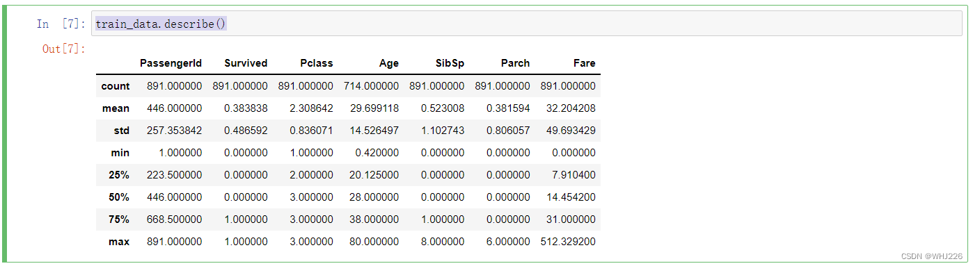
让我们检查一下目标是否确实是0或1:
train_data["Survived"].value_counts()运行结果如下:
0    549
1    342
Name: Survived, dtype: int64
现在让我们看一下所有的分类属性:
train_data["Pclass"].value_counts()运行结果如下:
3    491
1    216
2    184
Name: Pclass, dtype: int64train_data["Sex"].value_counts()运行结果如下:
male      577
female    314
Name: Sex, dtype: int64train_data["Embarked"].value_counts()运行结果如下:(该属性表示乘客上船地点)
S    644
C    168
Q     77
Name: Embarked, dtype: int64
C=Cherbourg, Q=Queenstown, S=Southampton.
现在让我们构建预处理管道。我们将构建DataframeSelector来从DataFrame中选择特定的属性:
from sklearn.base import BaseEstimator, TransformerMixin

# 选择数值列或分类列的类
# since Scikit-Learn doesn't handle DataFrames yet
class DataFrameSelector(BaseEstimator, TransformerMixin):
    def __init__(self, attribute_names):
        self.attribute_names = attribute_names
    def fit(self, X, y=None):
        return self
    def transform(self, X):
        return X[self.attribute_names]
让我们为数值属性构建管道:
from sklearn.pipeline import Pipeline
from sklearn.impute import SimpleImputer # Scikit-Learn 0.20+


num_pipeline = Pipeline([
        ("select_numeric", DataFrameSelector(["Age", "SibSp", "Parch", "Fare"])),
        ("imputer", SimpleImputer(strategy="median")),
    ])


num_pipeline.fit_transform(train_data)
运行结果如下:
array([[22.    ,  1.    ,  0.    ,  7.25  ],
       [38.    ,  1.    ,  0.    , 71.2833],
       [26.    ,  0.    ,  0.    ,  7.925 ],
       ...,
       [28.    ,  1.    ,  2.    , 23.45  ],
       [26.    ,  0.    ,  0.    , 30.    ],
       [32.    ,  0.    ,  0.    ,  7.75  ]])
这里,我们还需要一个用于字符串分类列的imputer(普通的SimpleImputer无法处理这些列):
class MostFrequentImputer(BaseEstimator, TransformerMixin):
    def fit(self, X, y=None):
        self.most_frequent_ = pd.Series([X[c].value_counts().index[0] for c in X],
                                        index=X.columns)
        return self
    def transform(self, X, y=None):
        return X.fillna(self.most_frequent_)
现在我们可以为分类属性构建管道:
from sklearn.preprocessing import OrdinalEncoder # just to raise an ImportError if Scikit-Learn < 0.20
from sklearn.preprocessing import OneHotEncoder

cat_pipeline = Pipeline([
        ("select_cat", DataFrameSelector(["Pclass", "Sex", "Embarked"])),
        ("imputer", MostFrequentImputer()),
        ("cat_encoder", OneHotEncoder(sparse=False)),
    ])


cat_pipeline.fit_transform(train_data)
运行结果如下:
array([[0., 0., 1., ..., 0., 0., 1.],
       [1., 0., 0., ..., 1., 0., 0.],
       [0., 0., 1., ..., 0., 0., 1.],
       ...,
       [0., 0., 1., ..., 0., 0., 1.],
       [1., 0., 0., ..., 1., 0., 0.],
       [0., 0., 1., ..., 0., 1., 0.]])
最后,让我们联合数值和分类管道:
现在我们有了一个很好的预处理管道,它可以提取原始数据并输出数值输入特征,我们可以将这些特征输入到任何我们想要的机器学习模型中。
X_train = preprocess_pipeline.fit_transform(train_data)
X_train
运行结果如下:
array([[22.,  1.,  0., ...,  0.,  0.,  1.],
       [38.,  1.,  0., ...,  1.,  0.,  0.],
       [26.,  0.,  0., ...,  0.,  0.,  1.],
       ...,
       [28.,  1.,  2., ...,  0.,  0.,  1.],
       [26.,  0.,  0., ...,  1.,  0.,  0.],
       [32.,  0.,  0., ...,  0.,  1.,  0.]])
别忘了标签:
y_train = train_data["Survived"]现在我们准备训练一个分类器。让我们从SVC开始:
from sklearn.svm import SVC

svm_clf = SVC(gamma="auto")
svm_clf.fit(X_train, y_train)
现在,我们的模型训练好了,让我们用它来对测试集进行预测:
X_test = preprocess_pipeline.transform(test_data)
y_pred = svm_clf.predict(X_test)
我们可以使用交叉验证来了解我们的模型有多好。
from sklearn.model_selection import cross_val_score

svm_scores = cross_val_score(svm_clf, X_train, y_train, cv=10)
svm_scores.mean()
运行结果如下:
0.7329588014981274超过73%的准确率,显然比随机概率高,但这不是一个很好的分数。所以让我们尝试建立一个准确率达到80%的模型。
我们尝试一下RandomForestClassifier:
from sklearn.ensemble import RandomForestClassifier

forest_clf = RandomForestClassifier(n_estimators=100, random_state=42)
forest_scores = cross_val_score(forest_clf, X_train, y_train, cv=10)
forest_scores.mean()
运行结果如下:
0.8126466916354558我们不只是看10个交叉验证折叠的平均准确率,让我们绘制每个模型的所有10个得分,以及一个突出显示分数上下四分之一的盒子图,以及显示得分程度。
import matplotlib.pyplot as plt

plt.figure(figsize=(8, 4))
plt.plot([1]*10, svm_scores, ".")
plt.plot([2]*10, forest_scores, ".")
plt.boxplot([svm_scores, forest_scores], labels=("SVM","Random Forest"))
plt.ylabel("Accuracy", fontsize=14)
plt.show()
运行结果如下:
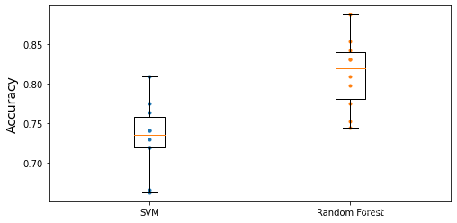
要进一步改善这个结果,我们可以使用交叉验证和网格搜索来比较更多的模型和优化超参数。
学习笔记——《机器学习实战:基于Scikit-Learn和TensorFlow》