WGAN原理及实现（pytorch版）

一、WGAN原理

1.1 原始GAN的缺陷

原始GAN通过最小化JS散度（Jensen-Shannon Divergence）训练生成器（Generator）和判别器（Discriminator），但存在两个关键问题：

1. 梯度消失：当真实分布 $P_r$ 和生成分布 $P_g$ 不重叠时，JS散度为常数 $\log 2$，导致梯度为0，无法更新生成器
2. 训练不稳定：判别器容易过拟合，生成器难以收敛

1.2 Wasserstein距离的引入

Wasserstein距离（Earth-Mover距离）衡量两个分布 ${\mathbb{P}}_r$（真实分布）和 ${\mathbb{P}}_g$（生成分布）之间的差异：

$W({\mathbb{P}}_r,{\mathbb{P}}_g)={\inf }_{\gamma \in \Pi ({\mathbb{P}}_r,{\mathbb{P}}_g)}{\mathbb{E}}_{(x,y)\sim \gamma }[\Vert x-y\Vert ]$，其中 $\Pi ({\mathbb{P}}_r,{\mathbb{P}}_g)$ 是联合分布集合，边缘分布分别为 ${\mathbb{P}}_r$ 和 ${\mathbb{P}}_g$

关键改进：即使两个分布支撑集不重叠，Wasserstein距离仍能提供有意义的梯度

直观解释：衡量将“概率质量”从 $P_r$ 搬运到 $P_g$ 的最小成本

1.3 Kantorovich-Rubinstein对偶

通过对偶形式将问题转化为：

$W({\mathbb{P}}_r,{\mathbb{P}}_g)={\sup }_{\Vert f{\Vert }_L\le 1}{\mathbb{E}}_{x\sim {\mathbb{P}}_r}[f(x)]-{\mathbb{E}}_{x\sim {\mathbb{P}}_g}[f(x)]$，其中 $f$ 是1-Lipschitz函数（满足 $|f(x)-f(y)|\le \Vert x-y\Vert$）

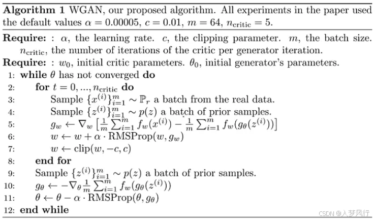
1.4 WGAN的优化目标

• 判别器（Critic）：拟合一个1-Lipschitz函数 $f_w$，最大化：
  $L_{\text{critic}}={\mathbb{E}}_{x\sim {\mathbb{P}}_r}[f_w(x)]-{\mathbb{E}}_{z\sim p(z)}[f_w(G_{\theta }(z))]$
• 生成器：最小化Wasserstein距离，即：
  $L_{\text{generator}}=-{\mathbb{E}}_{z\sim p(z)}[f_w(G_{\theta }(z))]$

关键点：

1. 判别器（称为Critic）输出为标量，无需Sigmoid激活
2. 通过权重裁剪（强制参数 $w$) 在 $[-c,c]$ 内）或梯度惩罚（WGAN-GP）近似Lipschitz约束

1.4 数学推导步骤

（1）原始Wasserstein距离

$W({\mathbb{P}}_r,{\mathbb{P}}_g)={\inf }_{\gamma }{\mathbb{E}}_{(x,y)\sim \gamma }[\Vert x-y\Vert ]$

（2）对偶形式推导

利用线性规划对偶性，转化为：$W({\mathbb{P}}_r,{\mathbb{P}}_g)={\sup }_{f\in \text{1-Lip}}{\mathbb{E}}_{x\sim {\mathbb{P}}_r}[f(x)]-{\mathbb{E}}_{x\sim {\mathbb{P}}_g}[f(x)]$

（3） 参数化近似
用神经网络 $f_w$ 近似 $f$，优化：${\max }_w{\mathbb{E}}_{x\sim {\mathbb{P}}_r}[f_w(x)]-{\mathbb{E}}_{z\sim p(z)}[f_w(G_{\theta }(z))]$

（4）生成器优化
固定$f_w$，生成器最小化：${\min }_{\theta }-{\mathbb{E}}_{z\sim p(z)}[f_w(G_{\theta }(z))]$

1.5 权重裁剪 vs 梯度惩罚

• 权重裁剪（原始WGAN）：
  强制参数 $w$ 在 $[-c,c]$ 内，但可能导致梯度消失或爆炸
• 梯度惩罚（WGAN-GP）：
  添加正则项： $\lambda {\mathbb{E}}_{\hat{x}\sim {\mathbb{P}}_{\hat{x}}}[(\Vert {\nabla }_{\hat{x}}{f}_w(\hat{x}){\Vert }_2-1{)}^2]$，其中 $\hat{x}$ 是真实样本和生成样本的随机插值

1.6 优势

1. 训练信号：Critic的损失值与生成样本质量相关（越低表示越真实）
2. 训练稳定性：避免模式崩溃（Mode Collapse）
3. 梯度有意义：即使分布不重叠，仍能提供有效梯度
4. 生成质量高：Wasserstein距离直接反映生成数据与真实数据的差异

1.7 总结

WGAN通过Wasserstein距离的优良性质，解决了传统GAN的训练难题。其数学核心在于对偶形式的转化和Lipschitz约束的实现，后续改进（如WGAN-GP）进一步提升了性能。

二、WGAN实现

2.1 导包

import torch
import torch.nn as nn
from torch.utils.data import DataLoader
from torch.utils.tensorboard import SummaryWriter
from torchvision import datasets, transforms
from torchvision.utils import save_image
import numpy as np

import os
import time
import matplotlib.pyplot as plt
from tqdm.notebook import tqdm  
from torchsummary import summary

# 判断是否存在可用的GPU
device=torch.device("cuda:0" if torch.cuda.is_available() else "cpu")

# 指定存放日志路径
writer=SummaryWriter(log_dir="./runs/wgan")

os.makedirs("./img/wgan_mnist", exist_ok=True) # 存放生成样本目录
os.makedirs("./model", exist_ok=True) # 模型存放目录

2.2 数据加载和处理

# 加载 MNIST 数据集
def load_data(batch_size=64,img_shape=(1,28,28)):
    transform = transforms.Compose([
        transforms.ToTensor(),  # 将图像转换为张量
        transforms.Normalize(mean=[0.5], std=[0.5])  # 归一化到[-1,1]
    ])
    
    # 下载训练集和测试集
    train_dataset = datasets.MNIST(root='./data', train=True, download=True, transform=transform)
    test_dataset = datasets.MNIST(root='./data', train=False, download=True, transform=transform)
    
    # 创建 DataLoader
    train_loader = DataLoader(dataset=train_dataset, batch_size=batch_size, num_workers=2,shuffle=True)
    test_loader = DataLoader(dataset=test_dataset, batch_size=batch_size, num_workers=2,shuffle=False)
    return train_loader, test_loader

2.3 构建生成器

class Generator(nn.Module):
    """生成器"""
    def __init__(self, latent_dim=100,img_shape=(1,28,28)):
        super(Generator,self).__init__()

        # 网络块
        def block(in_feat, out_feat, normalize=True):
            layers = [nn.Linear(in_feat, out_feat)]
            if normalize:
                layers.append(nn.BatchNorm1d(out_feat))
            layers.append(nn.LeakyReLU(negative_slope=0.2, inplace=True))
            return layers

        self.model = nn.Sequential(
            *block(latent_dim, 128, normalize=False),
            *block(128, 256),
            *block(256, 512),
            *block(512, 1024),
            nn.Linear(1024, int(np.prod(img_shape))),
            nn.Tanh() # 输出归一化到[-1,1] 
        )

        
    def forward(self,z): # 噪声z,2维[batch_size,latent_dim]
        gen_img=self.model(z) 
        gen_img=gen_img.view(gen_img.shape[0],*img_shape)
        return gen_img # 4维[batch_size,1,H,W]

2.4 构建判别器

class Discriminator(nn.Module):
    """判别器"""
    def __init__(self,img_shape=(1,28,28)):
        super(Discriminator, self).__init__()

        self.model = nn.Sequential(
                nn.Linear(int(np.prod(img_shape)), 512),
                nn.LeakyReLU(negative_slope=0.2, inplace=True),
                nn.Linear(512, 256),
                nn.LeakyReLU(negative_slope=0.2, inplace=True),
                nn.Linear(256, 1)
            )

    def forward(self,img): # 输入图片，4维[batc_size,1,H,W]
        img=img.view(img.shape[0], -1) 
        pred = self.model(img)
        return pred # 2维[batch_size,1] 

2.5 训练和保存模型

• WGAN算法流程
  
• 训练和保存

# 设置超参数
batch_size = 64
epochs = 200
lr= 0.00005
latent_dim=100 # 生成器输入噪声向量的长度(维数)
sample_interval=400 #每400次迭代保存生成样本

# WGAN的特别设置
num_iter_critic = 5
weight_clip_value = 0.01

# 设置图片形状1*28*28
img_shape = (1,28,28)

# 加载数据
train_loader,_= load_data(batch_size=batch_size,img_shape=img_shape)

# 实例化生成器G、判别器D
G=Generator().to(device)
D=Discriminator().to(device)

# 设置优化器
optimizer_G = torch.optim.RMSprop(G.parameters(), lr=lr)
optimizer_D = torch.optim.RMSprop(D.parameters(), lr=lr)

# 开始训练
batches_done=0
loader_len=len(train_loader) #训练集加载器的长度
for epoch in range(epochs):
    # 进入训练模式
    G.train()
    D.train()
    
    loop = tqdm(train_loader, desc=f"第{epoch+1}轮")
    for i, (real_imgs, _) in enumerate(loop):
        real_imgs=real_imgs.to(device)  # [B,C,H,W]

        
        # -----------------
        #  训练判别器
        # -----------------
        
        # 获取噪声样本[B,latent_dim）
        z=torch.normal(0,1,size=(real_imgs.shape[0],latent_dim),device=device)  #从正态分布中抽样
 
        # Step-1 计算判断器损失=判断真实图片损失+判断生成图片损失
        fake_imgs=G(z).detach()
        dis_loss=-torch.mean(D(real_imgs)) + torch.mean(D(fake_imgs))
       
        # Step-2 更新判别器参数
        optimizer_D.zero_grad() # 梯度清零
        dis_loss.backward() #反向传播,计算梯度
        optimizer_D.step()  #更新判别器 

        # Step-3 对判别器进行权重裁剪
        for p in D.parameters():
            p.data.clamp_(-weight_clip_value,weight_clip_value)

        # -----------------
        #  训练生成器
        # -----------------
 
        # 判别器每迭代 num_iter_critic 次,生成器迭代一次
        if i % num_iter_critic ==0 :

            gen_imgs=G(z).detach()

            # 更新生成器参数
            optimizer_G.zero_grad() #梯度清零
            gen_loss=-torch.mean(D(gen_imgs))
            gen_loss.backward() #反向传播,计算梯度
            optimizer_G.step()  #更新生成器  

             # 更新进度条
            loop.set_postfix(
                gen_loss=f"{gen_loss:.8f}",
                dis_loss=f"{dis_loss:.8f}"
            )
            

        # 每 sample_interval 次迭代保存生成样本
        if batches_done % sample_interval == 0:
            save_image(gen_imgs.data[:25], f"./img/wgan_mnist/{epoch}_{i}.png", nrow=5, normalize=True)
        batches_done += 1

print('总共训练用时: %.2f min' % ((time.time() - start_time)/60))

#仅保存模型的参数（权重和偏置）,灵活性高，可以在不同的模型结构之间加载参数
torch.save(G.state_dict(), "./model/WGAN_G.pth") 
torch.save(D.state_dict(), "./model/WGAN_D.pth") 

2.6 图片转GIF

from PIL import Image

def create_gif(img_dir="./img/wgan_mnist", output_file="./img/wgan_mnist/wgan_figure.gif", duration=100):
    images = []
    img_paths = [f for f in os.listdir(img_dir) if f.endswith(".png")]
    
    # 自定义排序：按 "x_y.png" 的 x 和 y 排序
    img_paths_sorted = sorted(
        img_paths,
        key=lambda x: (
            int(x.split('_')[0]),  # 第一个数字（如 0_400.png 的 0）
            int(x.split('_')[1].split('.')[0])  # 第二个数字（如 0_400.png 的 400）
        )
    )
    
    for img_file in img_paths_sorted:
        img = Image.open(os.path.join(img_dir, img_file))
        images.append(img)
    
    images[0].save(output_file, save_all=True, append_images=images[1:], 
                  duration=duration, loop=0)
    print(f"GIF已保存至 {output_file}")
create_gif()