卷积神经网络-EW帮帮网

想了解更多，请查看官方文档：点击查看

1. 基础层：

nn.Linear: 全连接层，用于定义线性变换
nn.Conv1d, nn.Conv2d, nn.Conv3d: 1D、2D 和 3D 卷积层
nn.MaxPool1d, nn.MaxPool2d, nn.MaxPool3d: 最大池化层
nn.AvgPool1d, nn.AvgPool2d, nn.AvgPool3d: 平均池化层

2. 激活函数：

nn.ReLU: ReLU（Rectified Linear Unit）激活函数
nn.Tanh: 双曲正切激活函数
nn.Sigmoid: Sigmoid 激活函数
nn.Softmax: Softmax 激活函数

3. 正则化层：

nn.Dropout: 随机失活，用于防止过拟合
nn.BatchNorm1d, nn.BatchNorm2d, nn.BatchNorm3d: 批标准化层

8类卷积操作

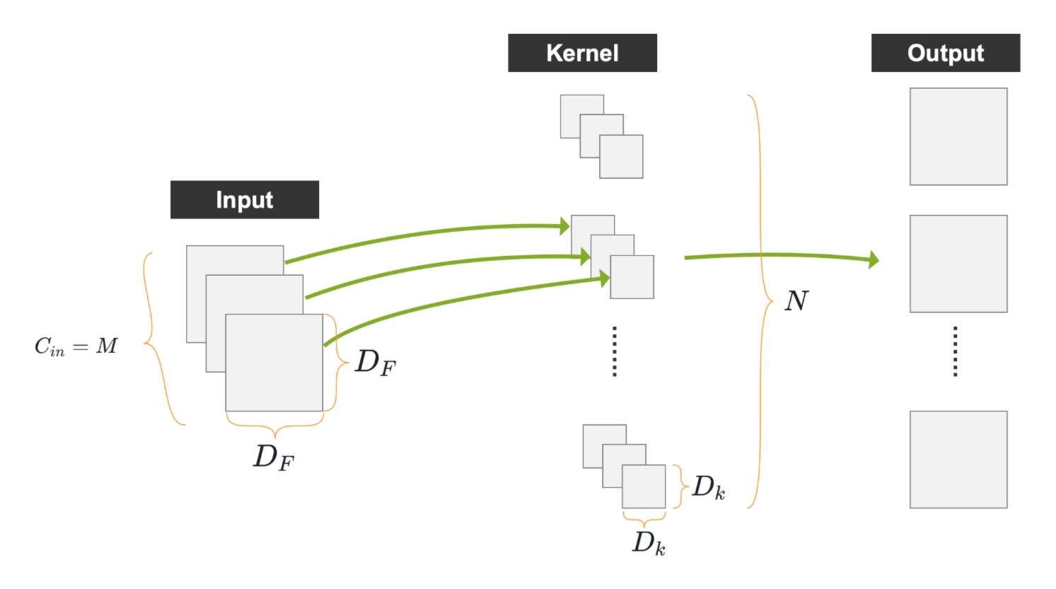
1、（Vanilla）Convolution (普通)卷积

卷积输出的尺寸的计算公式：

$W\_out = \frac{W_{in} + 2P_w - K_w}{S_w} + 1$
$H\_out = \frac{H_{in} +2P_h - K_h}{S_h} + 1$

其中，输入的尺寸为 ( $W_{\text{in}}, H_{\text{in}}$ )，卷积核的尺寸为 ( $K_w, K_h$ )，步幅为( $S_w, S_h$ )，填充为( $P_w, P_h$ )，输出的尺寸为( $W_{\text{out}}, H_{\text{out}}$ )

2、Group Convolution 分组卷积

Group convolution（分组卷积）最早是在AlexNet（Alex Krizhevsky等人于2012年提出的深度神经网络模型）中引入的。在 AlexNet中，作者们使用了分组卷积来将计算分布到多个GPU上。

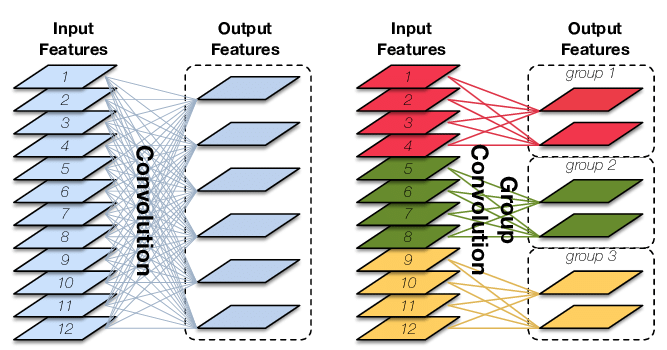
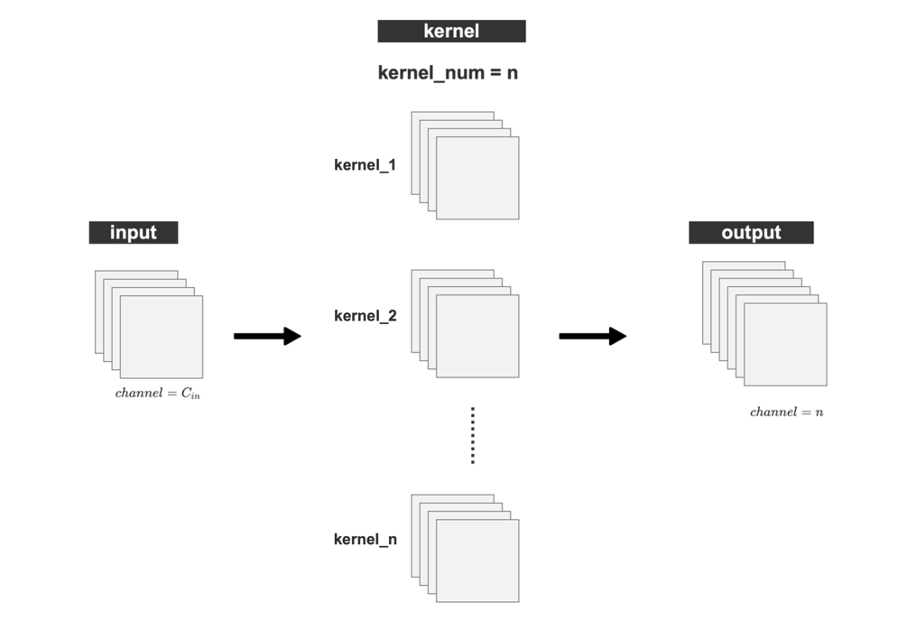
Group Convolution ：将输入 feature map 在 channel 的维度上进行分组，然后再对每个分组分别进行卷积操作

Group Convolution 可减小参数量。如下图，假设输入尺寸为 $C_{in} \times H \times W$ ，卷积核尺寸为 $K \times K$ ，输出的 Channel 数为 n，我们分别使用普通卷积和分组卷积来进行操作，并对比两种卷积方式的参数量

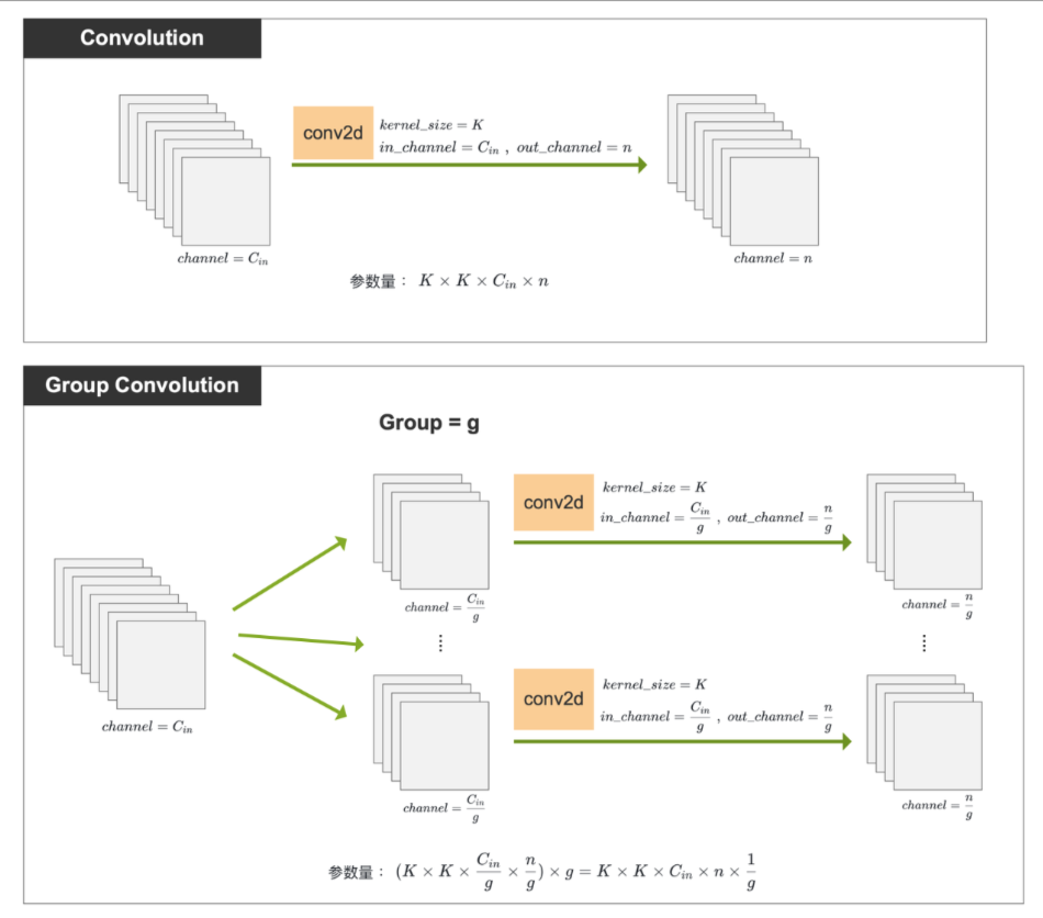
由上可知：Group Convolution 的参数量是普通卷积参数量的 $\frac{1}{g}$

** 特殊情况：当分组数量 g 等于输入channel 数量，Group Convolution 就等价于 Depthwise Convolution。

代码示例：

使用 torch.nn.conv2d()，并通过参数 groups 指定组数
in_channels 和 out_channels 都必须可以被 groups 整除，否则会报错，类似：ValueError: in_channels must be divisible by groups

import torch
import torch.nn as nn

conv = nn.Conv2d(in_channels=10, out_channels=15, kernel_size=3, groups=5, stride=1, padding=1)
output = conv(torch.rand(1, 10, 20, 20))
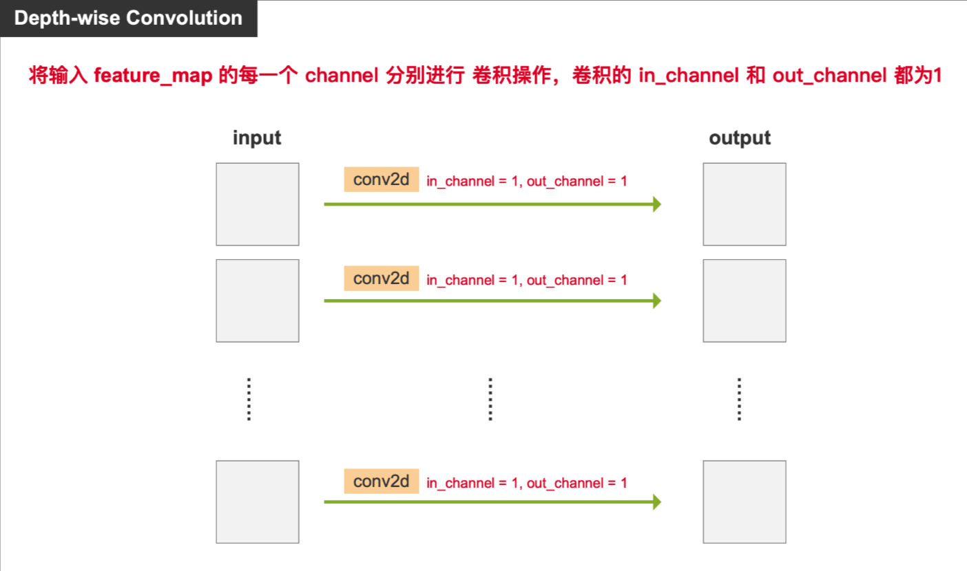
print(output.shape)   # torch.Size([1, 15, 20, 20])

3、Depth-wise Convolution 逐深度卷积

将输入图像的每一个 channel 分别进行卷积操作，卷积的 in_channel 和 out_channel 都为1

使用 DW Convolution，输出的 channel 和输入 channel一样
当 group Convolution 的组数等于输入 channel 时，即 $g = C_{in}$ 时，就是 Depth-wise convolution
优点：参数量和计算量小

代码示例：将 nn.Conv2d 的参数 out_channels 和 groups 都设置为等于 in_channels

import torch
import torch.nn as nn

conv = nn.Conv2d(in_channels=10, out_channels=10, kernel_size=3, groups=10, stride=1, padding=1)
output = conv(torch.rand(1, 10, 20, 20))
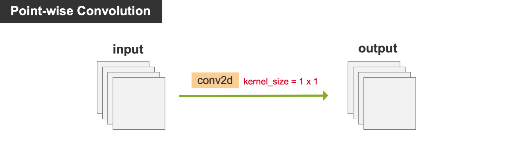
print(output.shape)   # torch.Size([1, 10, 20, 20])

4、Point-wise Convolution 逐点卷积

就是普通卷积，只不过 kernel_size=1x1，也就是我们经常看到的 conv 1x1，它通常用来组合通道之间的特征信息

优点：参数量和计算量小

代码示例：将 nn.Conv2d 的参数 kernel_size 设置为等于 1

import torch
import torch.nn as nn

conv = nn.Conv2d(in_channels=10, out_channels=10, kernel_size=1, stride=1)
output = conv(torch.rand(1, 10, 20, 20))
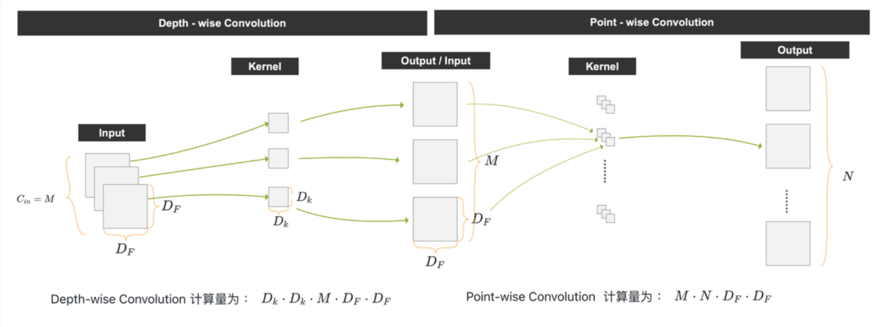
print(output.shape)   # torch.Size([1, 10, 20, 20])

5、Depth-wise Separable Convolution 深度可分离卷积

Depth-wise Separable Convolution（深度可分离卷积）最早是由Google的研究团队在2014年提出的。该方法首次出现在论文《MobileNets: Efficient Convolutional Neural Networks for Mobile Vision Applications》中

Depth-wise Separable Convolution 就是先做一个 Depth-wise Convolution ，后面再做一个 Point-wise Convolution （或者先做一个 Depth-wise Convolution ，后面再做一个 Point-wise Convolution ）

他的优势是极大的减小了卷积的计算量

（1）对于普通卷积而言，计算量为 (公式1)： $D_k \cdot D_k \cdot M \cdot N \cdot D_F \cdot D_F$

（2）Depth-wise Separable Convolution，计算量为（公式2）： $D_k \cdot D_k \cdot M \cdot D_F \cdot D_F + M \cdot N \cdot D_F \cdot D_F$

其中：

对于 Depth-wise Convolution，计算量为： $D_k \cdot D_k \cdot M \cdot D_F \cdot D_F$
对于 Point-wise Convolution ，计算量为： $M \cdot N \cdot D_F \cdot D_F$

为了对比普通卷积和深度可分离卷积的计算量，我们用公式(2) 除以公式(1) ：

$\frac{D_k \cdot D_k \cdot M \cdot D_F \cdot D_F + M \cdot N \cdot D_F \cdot D_F}{D_k \cdot D_k \cdot M \cdot N \cdot D_F \cdot D_F} = \frac{1}{N} + \frac{1}{D_k^2}$

通常，我们在使用卷积的时候，使用的最多的还是 $3 \times 3$ 的卷积，即 $D_k = 3$ ，所以，上面的公式(3)，一般等于：

$\frac{1}{N} + \frac{1}{D_k^2} = \frac{1}{N} + \frac{1}{9}$

所以，理论上，普通卷积的计算量是深度可分离卷积计算量的 8倍～ 9倍

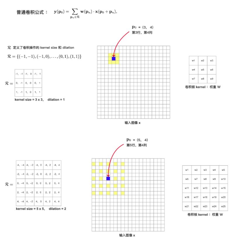
6、Dilation Convolution 膨胀卷积

Dilation Convolution 称为空洞卷积或膨胀卷积，其通过在卷积核的元素之间引入间隔（dilation），从而增大了卷积核的感受野。

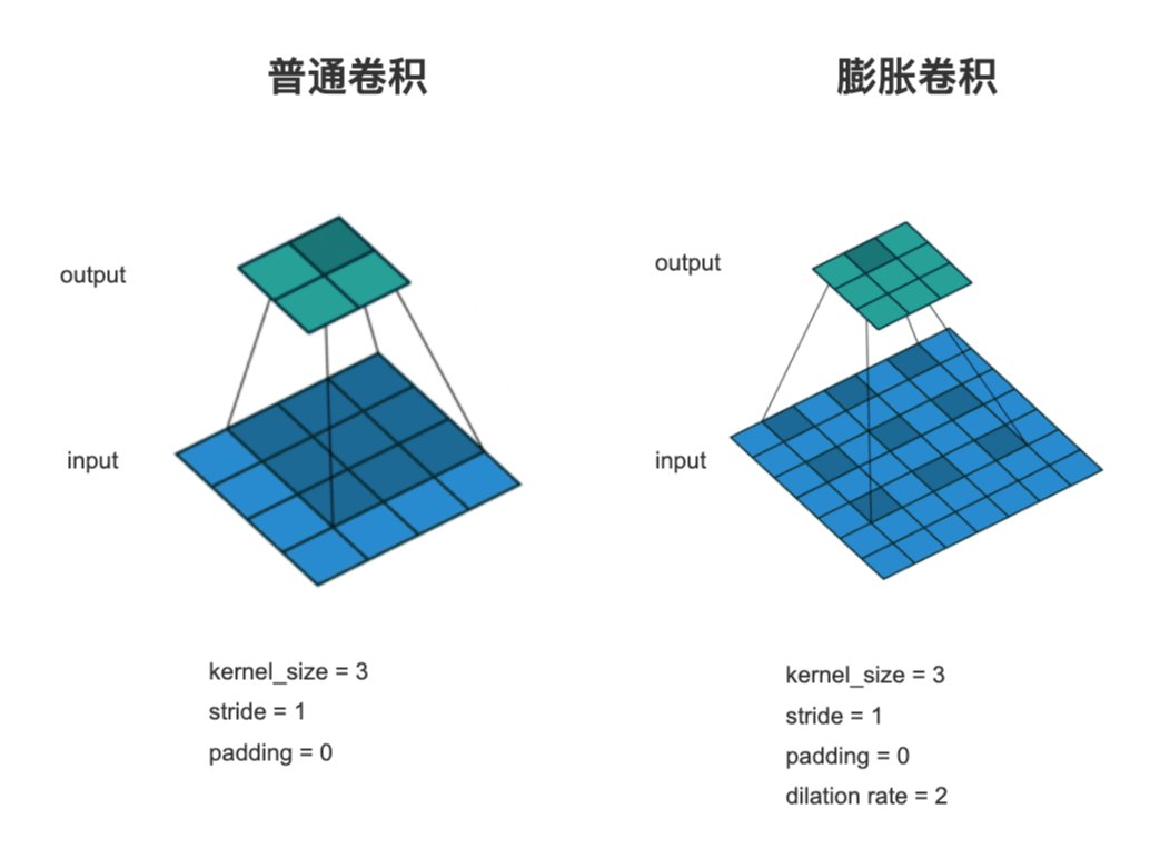
当 dilation=1 时，是普通卷积
当 dilation=2 时，卷积核元素中间间隔一个像素
依此类推

代码示例：指定参数 dilation

import torch
import torch.nn as nn

conv = nn.Conv2d(in_channels=10, out_channels=10, kernel_size=3, stride=1, padding=2, dilation=2)
output = conv(torch.rand(1, 10, 20, 20))
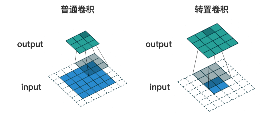
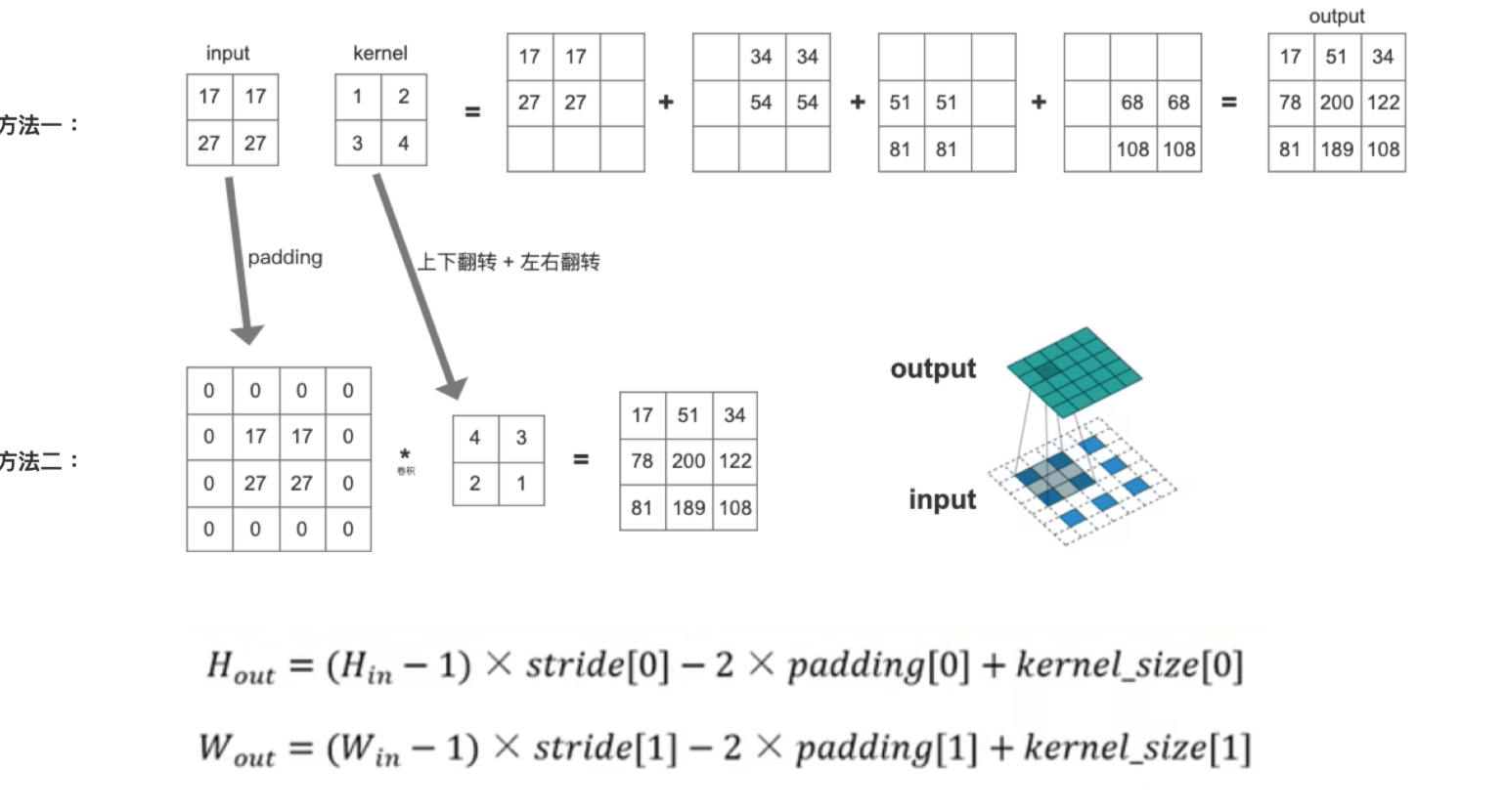
print(output.shape)   # torch.Size([1, 10, 20, 20])

7、Transposed Convolution 转置卷积

转置卷积也是卷积，只不过转置卷积是一种上采样操作

如下图的转置卷积所示，输入图像尺寸为 2x2，输出图像的尺寸为 4x4

（1）如何设置转置卷积的 stride 和 padding

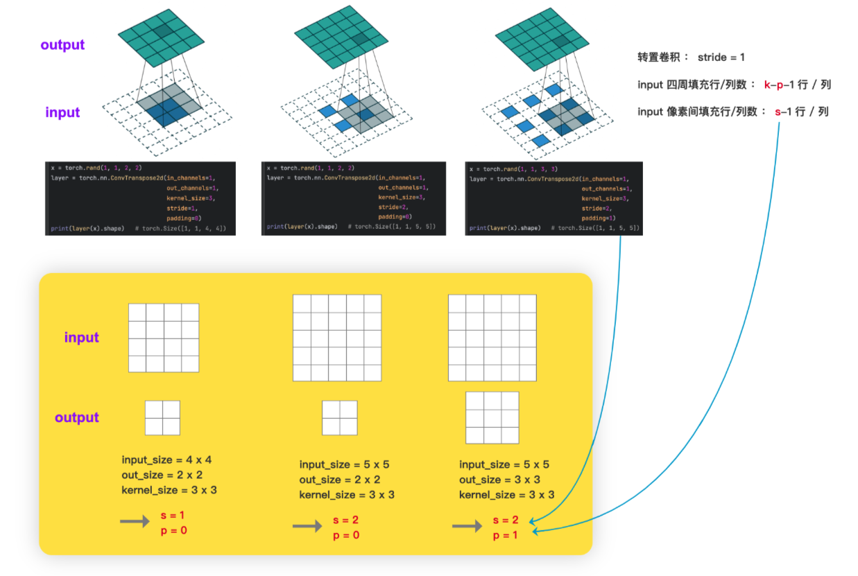
（2）已知 input 和 kernel，求 output

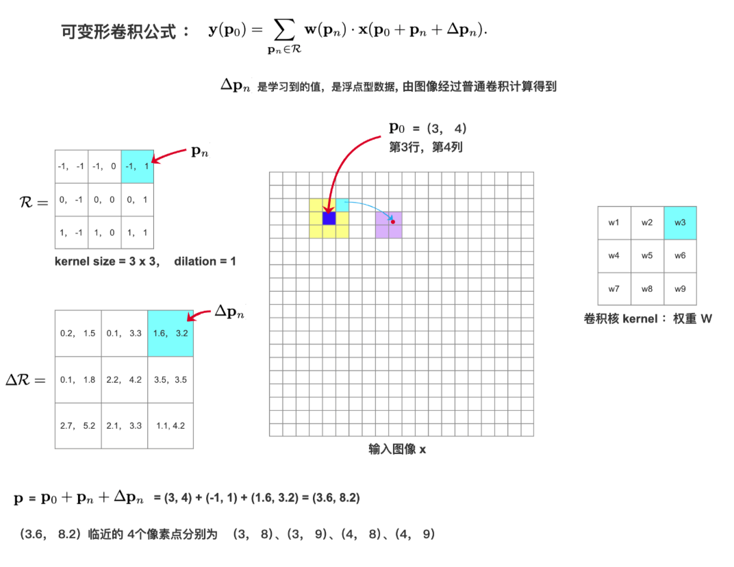
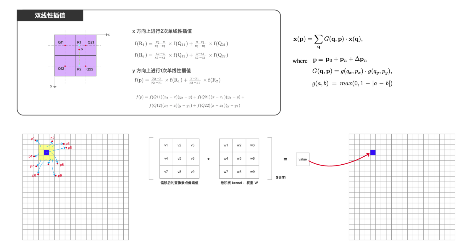
8、Deformable Convolution 可变形卷积

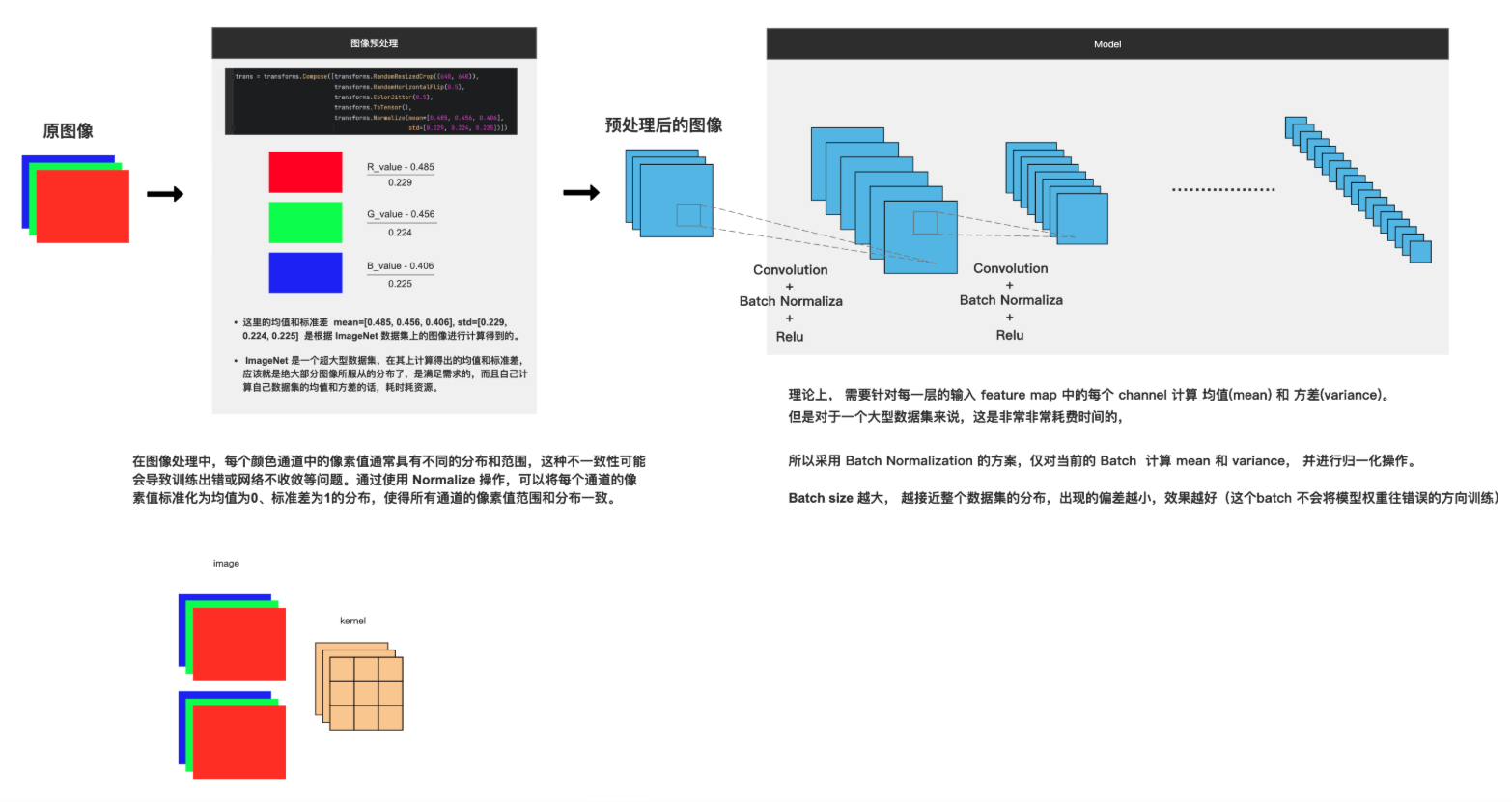
BatchNormlization

1、作用

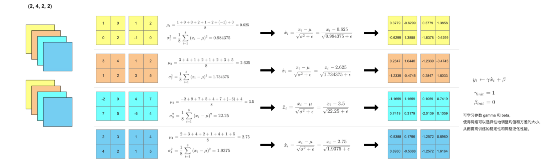
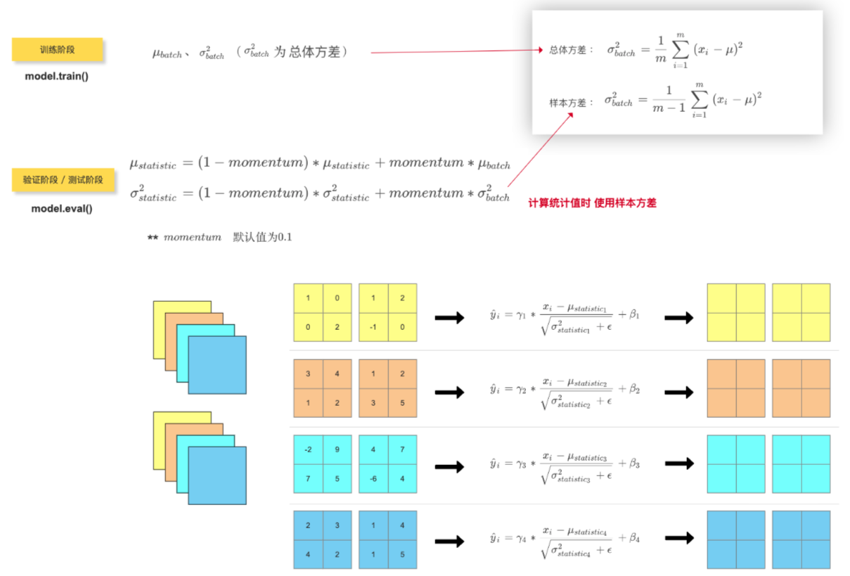
2、计算方式

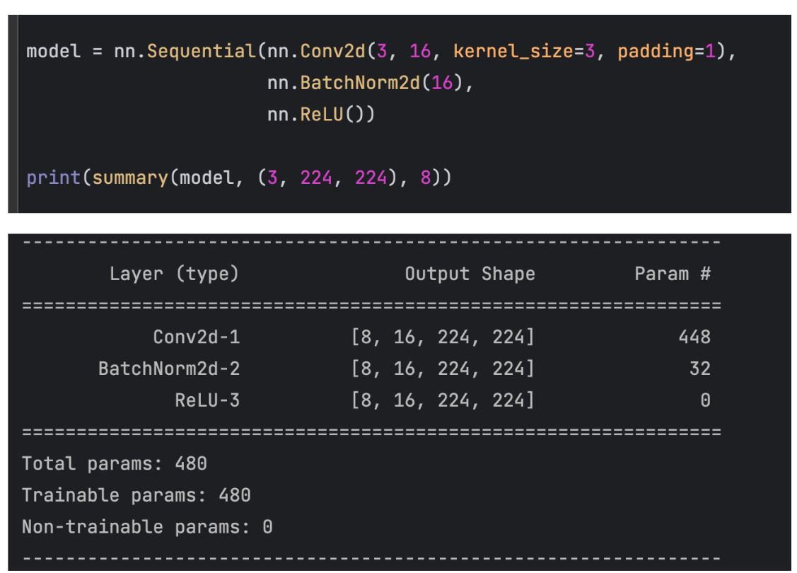
3、查看BN 层中的参数数量

BN层中有 weight 和 bias 两个参数（也就是上面计算方式中的 gamma 和 beta）

如下代码中，BN层输入的 channel数为 16，每个 channel 有 2个可学习参数，一共有32个可学习参数

4、验证阶段 / 测试阶段的Batch Normalization

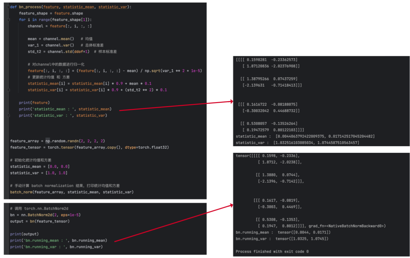
证明一下，自己手动计算出的 BN层的统计均值和统计方差和调用 nn.BatchNorm() 计算结果一致

import numpy as np
import torch.nn as nn
import torch


def batch_norm(feature, statistic_mean, statistic_var):
    feature_shape = feature.shape
    for i in range(feature_shape[1]):
        channel = feature[:, i, :, :]
        mean = channel.mean()   # 均值
        std_1 = channel.std()   # 总体标准差
        std_t2 = channel.std(ddof=1)  # 样本标准差
        # 对channel中的数据进行归一化
        feature[:, i, :, :] = (channel - mean) / np.sqrt(std_1 ** 2 + 1e-5)
        # 更新统计均值 和 方差
        statistic_mean[i] = statistic_mean[i] * 0.9 + mean * 0.1
        statistic_var[i] = statistic_var[i] * 0.9 + (std_t2 ** 2) * 0.1

    print(feature)
    print('statistic_mean : ', statistic_mean)
    print('statistic_var : ', statistic_var)



feature_array = np.random.randn(2, 2, 2, 2)
feature_tensor = torch.tensor(feature_array.copy(), dtype=torch.float32)

# 初始化统计均值和方差
statistic_mean = [0.0, 0.0]
statistic_var = [1.0, 1.0]

# 手动计算 batch normalization 结果，打印统计均值和方差
batch_norm(feature_array, statistic_mean, statistic_var)

# 调用 torch.nn.BatchNorm2d
bn = nn.BatchNorm2d(2, eps=1e-5)
output = bn(feature_tensor)

print(output)
print('bn.running_mean : ', bn.running_mean)
print('bn.running_var : ', bn.running_var)

5、模型中BN层的使用节点

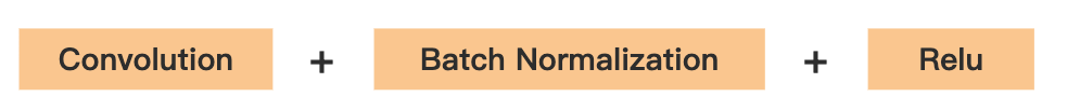
这种顺序之所以能够效果良好，是因为批量归一化能够使得输入分布均匀，而 ReLU 又能够将分布中的负值清除，从而达到更好的效果。

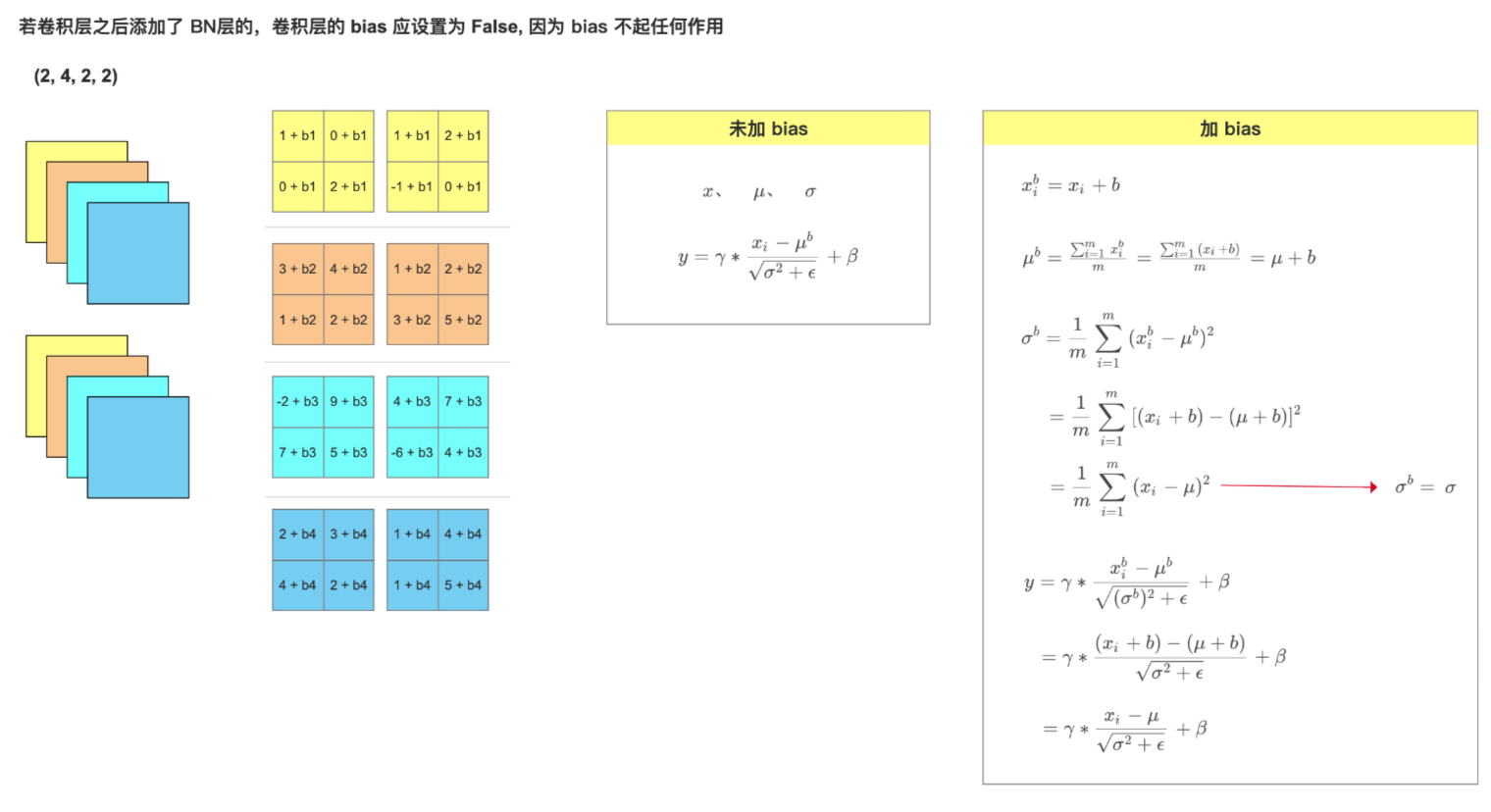
6、BN层对卷积层的影响

BatchNorm、LayerNorm、GroupNorm

1、BatchNorm

BatchNorm、LayerNorm 和 GroupNorm 都是深度学习中常用的归一化方式。

它们通过将输入归一化到均值为 0 和方差为 1 的分布中，来防止梯度消失和爆炸，并提高模型的泛化能力。

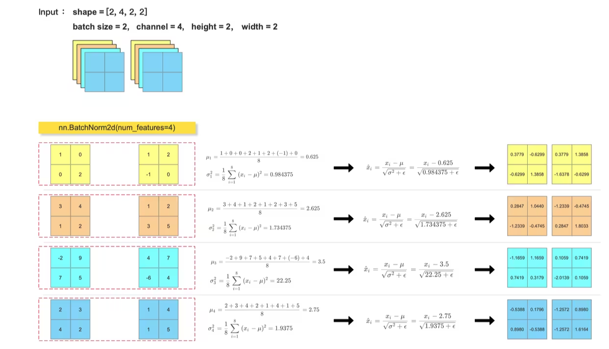
对比手动计算的 BN层输出结果和调用 nn.BatchNorm() 的输出结果

import torch
import torch.nn as nn
import numpy as np

feature_array = np.array([[[[1, 0],  [0, 2]],
                           [[3, 4],  [1, 2]],
                           [[-2, 9], [7, 5]],
                           [[2, 3],  [4, 2]]],

                          [[[1, 2],  [-1, 0]],
                            [[1, 2], [3, 5]],
                            [[4, 7], [-6, 4]],
                            [[1, 4], [1, 5]]]], dtype=np.float32)

feature_tensor = torch.tensor(feature_array.copy(), dtype=torch.float32)
bn_out = nn.BatchNorm2d(num_features=4, eps=1e-5)(feature_tensor)
print(bn_out)

for i in range(feature_array.shape[1]):
    channel = feature_array[:, i, :, :]
    mean = feature_array[:, i, :, :].mean()
    var = feature_array[:, i, :, :].var()
    print(mean)
    print(var)

    feature_array[:, i, :, :] = (feature_array[:, i, :, :] - mean) / np.sqrt(var + 1e-5)
print(feature_array)

2、LayerNorm

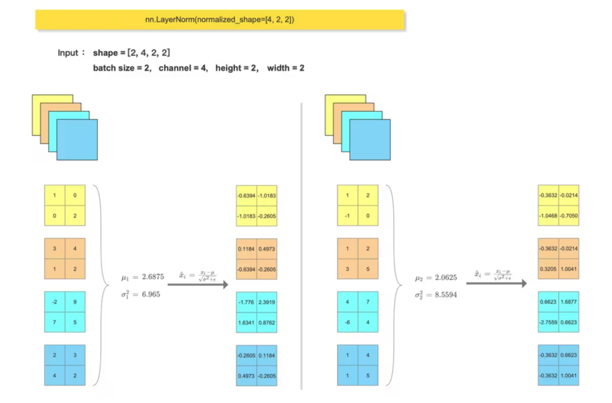
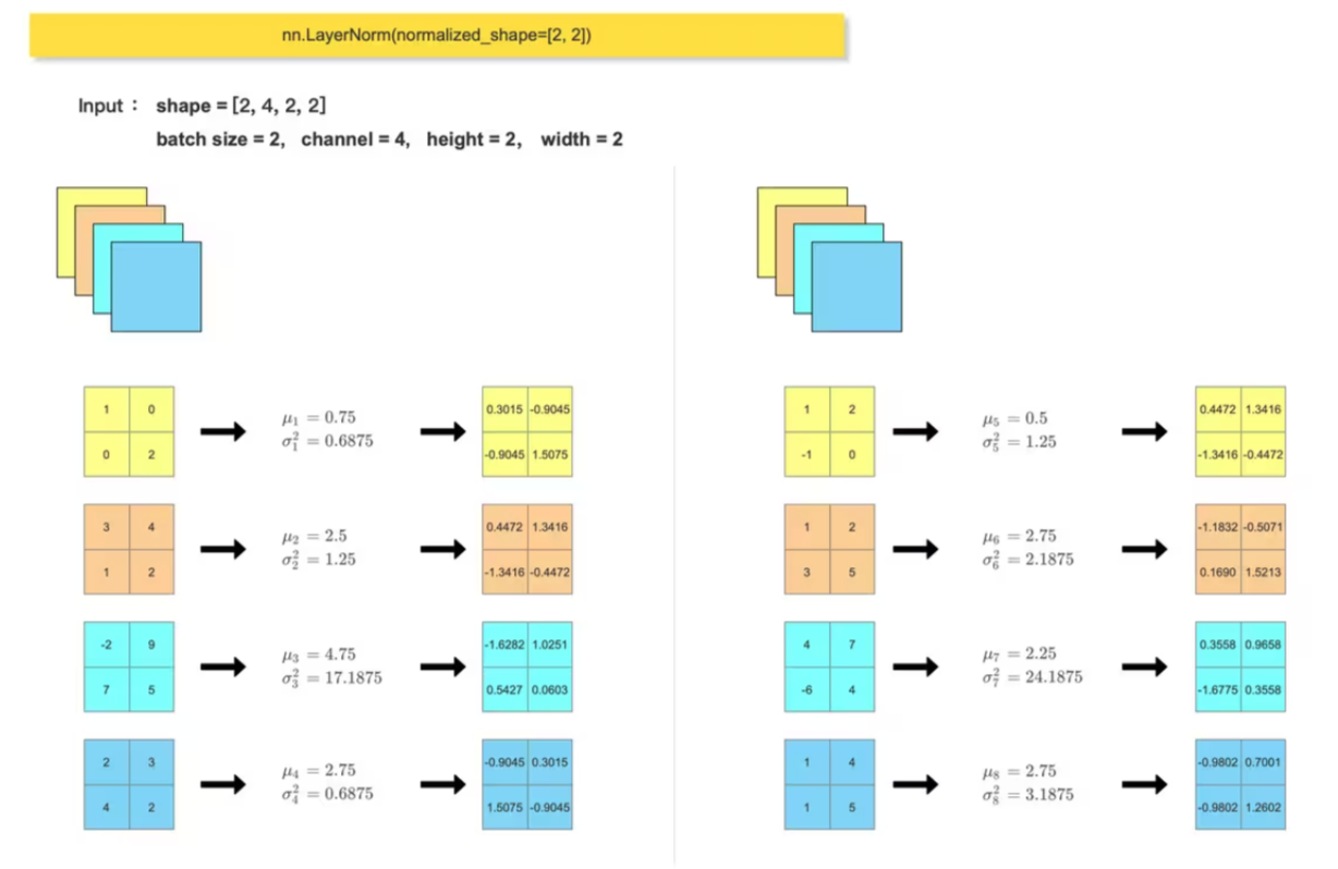
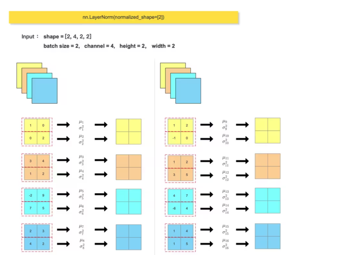
Transformer block 中会使用到 LayerNorm ，一般输入尺寸形为：（batch_size, token_num, dim），会在最后一个维度做归一化： nn.LayerNorm(dim)

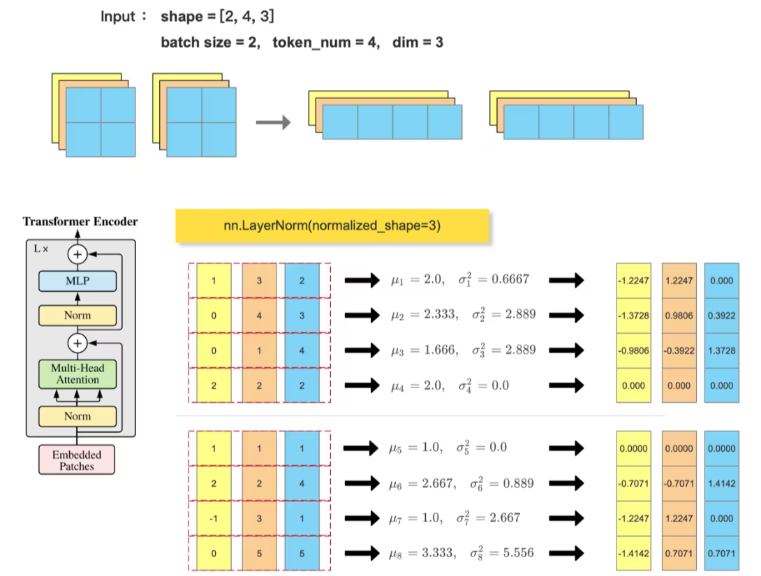
对比手动计算的 LN层输出结果和调用 nn.LayerNorm() 的输出结果

import torch
import torch.nn as nn
import numpy as np

feature_array = np.array([[[[1, 0],  [0, 2]],
                           [[3, 4],  [1, 2]],
                           [[2, 3],  [4, 2]]],

                          [[[1, 2],  [-1, 0]],
                            [[1, 2], [3, 5]],
                            [[1, 4], [1, 5]]]], dtype=np.float32)


feature_array = feature_array.reshape((2, 3, -1)).transpose(0, 2, 1)
feature_tensor = torch.tensor(feature_array.copy(), dtype=torch.float32)

ln_out = nn.LayerNorm(normalized_shape=3)(feature_tensor)
print(ln_out)

b, token_num, dim = feature_array.shape
feature_array = feature_array.reshape((-1, dim))
for i in range(b*token_num):
    mean = feature_array[i, :].mean()
    var = feature_array[i, :].var()
    print(mean)
    print(var)

    feature_array[i, :] = (feature_array[i, :] - mean) / np.sqrt(var + 1e-5)
print(feature_array.reshape(b, token_num, dim))

3、GroupNorm

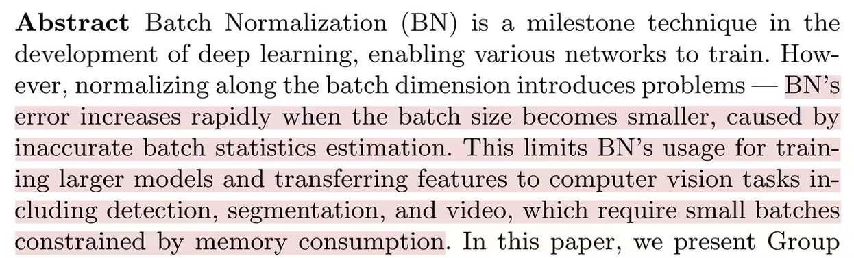
batch size 过大或过小都不适合使用 BN，而是使用 GN。

（1）当 batch size 过大时，BN 会将所有数据归一化到相同的均值和方差。这可能会导致模型在训练时变得非常不稳定，并且很难收敛。

（2）当 batch size 过小时，BN 可能无法有效地学习数据的统计信息。

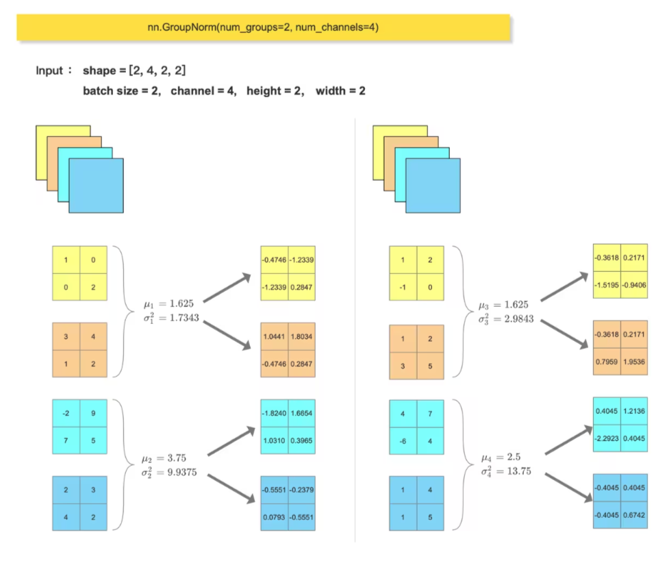
对比手动计算的 GN层输出结果和调用 nn.GroupNorm() 的输出结果

import torch
import torch.nn as nn
import numpy as np

feature_array = np.array([[[[1, 0],  [0, 2]],
                           [[3, 4],  [1, 2]],
                           [[-2, 9], [7, 5]],
                           [[2, 3],  [4, 2]]],

                          [[[1, 2],  [-1, 0]],
                            [[1, 2], [3, 5]],
                            [[4, 7], [-6, 4]],
                            [[1, 4], [1, 5]]]], dtype=np.float32)

feature_tensor = torch.tensor(feature_array.copy(), dtype=torch.float32)
gn_out = nn.GroupNorm(num_groups=2, num_channels=4)(feature_tensor)
print(gn_out)

feature_array = feature_array.reshape((2, 2, 2, 2, 2)).reshape((4, 2, 2, 2))

for i in range(feature_array.shape[0]):
    channel = feature_array[i, :, :, :]
    mean = feature_array[i, :, :, :].mean()
    var = feature_array[i, :, :, :].var()
    print(mean)
    print(var)

    feature_array[i, :, :, :] = (feature_array[i, :, :, :] - mean) / np.sqrt(var + 1e-5)
feature_array = feature_array.reshape((2, 2, 2, 2, 2)).reshape((2, 4, 2, 2))
print(feature_array)

附

nn.LayerNorm 参数 num_features 的使用

卷积神经网络