一·图形拼接
逻辑
- 导入必要的库
python
import cv2
import numpy as np
import sys
导入cv2库用于图像处理,numpy库用于数值计算,sys库用于与 Python 解释器进行交互,例如退出程序。
- 定义图像显示函数
def cv_show(name, img):
    cv2.imshow(name, img)
    cv2.waitKey(0)
cv_show函数用于在窗口中显示图像,并等待用户按键关闭窗口。它接受两个参数,name是窗口名称,img是要显示的图像。
- 定义特征检测与描述函数
python
def detectAndDescribe(image):
    gray = cv2.cvtColor(image, cv2.COLOR_BGR2GRAY)
    descriptor = cv2.SIFT_create()
    (kps, des) = descriptor.detectAndCompute(gray, None)
    kps_float = np.float32([kp.pt for kp in kps])
    return (kps, kps_float, des)
- 函数
detectAndDescribe接受一个图像作为输入。 - 首先将彩色图像转换为灰度图像,因为 SIFT 算法通常在灰度图像上进行操作。
- 创建 SIFT 特征提取器对象
descriptor。 - 使用
descriptor.detectAndCompute方法同时检测图像中的关键点并计算这些关键点的描述符。kps是关键点列表,des是描述符。 - 将关键点的坐标转换为
numpy的float32类型数组kps_float,方便后续计算。 - 最后返回关键点集
kps、关键点坐标数组kps_float以及描述符des。
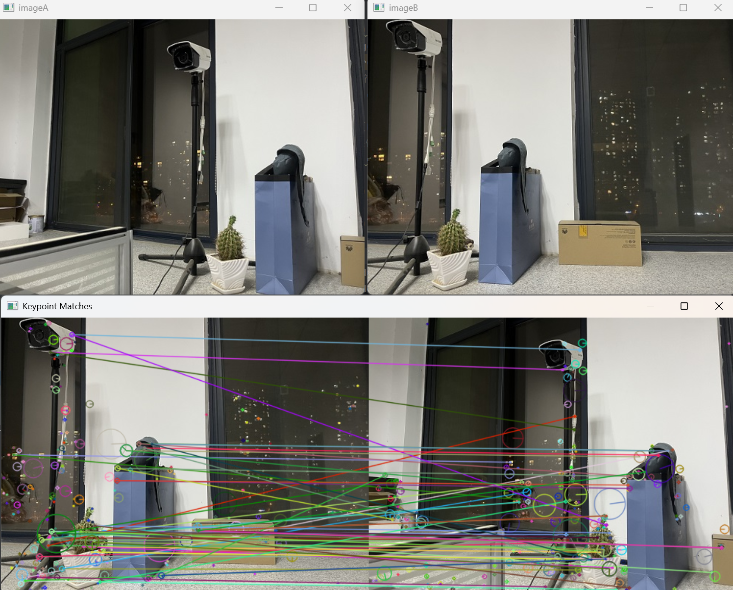
- 读取并显示拼接图片
imageA = cv2.imread("1.jpg")
cv_show('imageA', imageA)
imageB = cv2.imread("2.jpg")
cv_show('imageB', imageB)
使用cv2.imread分别读取两张要拼接的图像1.jpg和2.jpg,并通过cv_show函数在不同窗口中显示原始图像,让用户可以直观查看。
- 计算图片特征点及描述符
python
(kpsA, kps_floatA, desA) = detectAndDescribe(imageA)
(kpsB, kps_floatB, desB) = detectAndDescribe(imageB)
对图像imageA和imageB分别调用detectAndDescribe函数,获取它们的关键点集、关键点坐标数组以及描述符。
- 建立匹配器并进行特征匹配
python
matcher = cv2.BFMatcher()
rawMatches = matcher.knnMatch(desB, desA, 2)
good = []
matches = []
for m in rawMatches:
    if len(m) == 2 and m[0].distance < 0.65 * m[1].distance:
        good.append(m)
        matches.append((m[0].queryIdx, m[0].trainIdx))
- 创建
cv2.BFMatcher对象matcher,这是一个暴力匹配器,用于匹配两个图像的特征描述符。虽然代码注释提到在匹配大型训练集合时FlannBasedMatcher速度更快,但这里使用了BFMatcher。 - 使用
matcher.knnMatch方法对图像imageB和imageA的描述符进行 K 近邻匹配,k = 2表示为图像imageB的每个描述符在图像imageA的描述符中寻找最近的两个匹配。 - 遍历所有匹配结果
rawMatches,通过比率测试筛选出较好的匹配点。当最近距离与次近距离的比值小于 0.65 时,认为该匹配是一个好的匹配,将其添加到good列表中,并将匹配点在两个图像中的索引添加到matches列表中。
- 绘制匹配点连线并显示
python
vis = cv2.drawMatchesKnn(imageB, kpsB, imageA, kpsA, good, None,flags=cv2.DRAW_MATCHES_FLAGS_DRAW_RICH_KEYPOINTS)
cv_show("Keypoint Matches", vis)
使用cv2.drawMatchesKnn函数绘制匹配点之间的连线。该函数接受图像imageB及其关键点kpsB、图像imageA及其关键点kpsA、筛选后的匹配对good等参数。flags=cv2.DRAW_MATCHES_FLAGS_DRAW_RICH_KEYPOINTS参数表示绘制更丰富的关键点信息。绘制结果保存在vis中,然后通过cv_show函数在名为Keypoint Matches的窗口中显示绘制了匹配连线的图像。
- 透视变换与图像拼接
python
if len(matches) > 4:
    ptsB = np.float32([kps_floatB[i] for (i, _) in matches])
    ptsA = np.float32([kps_floatA[i] for (_, i) in matches])

    (H, mask) = cv2.findHomography(ptsB, ptsA, cv2.RANSAC, 10)
else:
    print('图片未找到4个以上的匹配点')
    sys.exit()

result = cv2.warpPerspective(imageB, H, (imageB.shape[1] + imageA.shape[1], imageB.shape[0]))
cv_show('resultB', result)
result[0:imageA.shape[0], 0:imageA.shape[1]] = imageA
cv_show('result', result)
- 当筛选后的匹配对数量大于 4 时,可以计算视角变换矩阵。
- 从
matches列表中提取图像imageB和imageA的匹配点坐标,分别存储在ptsB和ptsA中。 - 使用
cv2.findHomography函数计算透视变换矩阵H,这里使用cv2.RANSAC方法,并设置最大允许重投影错误阈值为 10。RANSAC方法可以有效剔除误匹配点,提高变换矩阵的准确性。 - 如果匹配点数量小于 4,则打印提示信息并退出程序。
- 使用计算得到的透视变换矩阵
H,对图像imageB进行透视变换,得到变换后的图像result。变换后的图像宽度是两张原始图像宽度之和,高度与图像imageB相同。 - 将图像
imageA放置在result图像的最左端,完成图像拼接。 - 最后通过
cv_show函数分别显示变换后的图像resultB和拼接后的最终图像result。
代码
import cv2
import numpy as np
import sys
def cv_show(name, img):
    cv2.imshow(name, img)
    cv2.waitKey(0)
def detectAndDescribe(image):
    gray = cv2.cvtColor(image, cv2.COLOR_BGR2GRAY)  # 将彩色图片转换成灰度图
    descriptor = cv2.SIFT_create()  # 建立SIFT生成器
    # 检测SIFT特征点,并计算描述符,第二个参数为掩膜
    (kps, des) = descriptor.detectAndCompute(gray, None)
    # 将结果转换成NumPy数组
    kps_float = np.float32([kp.pt for kp in kps])
    # kp.pt 包含两个值,分别是关键点在图像中的 x 和 y 坐标。这些坐标通常是浮点数,可以精确地描述关键点在图像中的位置。
    return (kps, kps_float, des)  # 返回特征点集,及对应的描述特征
'''读取拼接图片'''
imageA = cv2.imread("1.jpg")
cv_show('imageA', imageA)
imageB = cv2.imread("2.jpg")
cv_show('imageB', imageB)
'''计算图片特征点及描述符'''
(kpsA, kps_floatA, desA) = detectAndDescribe(imageA)
(kpsB, kps_floatB, desB) = detectAndDescribe(imageB)
'''建立暴力匹配器BFMatcher,在匹配大型训练集合时使用FlannBasedMatcher速度更快。'''
matcher = cv2.BFMatcher()
# knnMatch(queryDescriptors, trainDescriptors, k, mask=None, compactResult=None)
# 使用KNN检测来自A、B图的SIFT特征匹配对,参数说明:
# queryDescriptors:匹配图像A的描述符
# trainDescriptors:匹配图像B的描述符
# k:最佳匹配的描述符个数。一般K=2。
# 返回的数据结构描述:
# distance:匹配的特征点描述符的欧式距离,数值越小也就说明俩个特征点越相近。
# queryIdx:测试图像的特征点描述符的下标(第几个特征点描述符),同时也是描述符对应特征点的下标。
# trainIdx:样本图像的特征点描述符下标, 同时也是描述符对应特征点的下标。
rawMatches = matcher.knnMatch(desB, desA, 2)
good = []
matches = []
for m in rawMatches:
    # 当最近距离跟次近距离的比值小于0.65值时,保留此匹配对
    if len(m) == 2 and m[0].distance < 0.65 * m[1].distance:
        good.append(m)
        # 存储两个点在featuresA, featuresB中的索引值
        matches.append((m[0].queryIdx, m[0].trainIdx))
# print(len(good))
# print(matches)

# drawMatchesKnn(img1, keypoints1, img2, keypoints2, matches1to2, outImg, matchColor=None, singlePointColor=None, matchesMask=None, flags=None)绘制匹配图片
# 参数:img1:第一张原始图像。
# keypoints1:第一张原始图像的关键点。
# img2:第二张原始图像。
# keypoints2:第二张原始图像的关键点。
# matches1to2:从第一个图像到第二个图像的匹配,这意味着keypoints1[i]在keypoints2[Matches[i]中有一个对应的点。
# outImg:绘制结果图像。
# matchColor:匹配连线与关键点点的颜色,当matchColor == Scalar::all(-1)时,代表取随机颜色。
# singlePointColor:没有匹配项的关键点的颜色,当singlePointColor == Scalar::all(-1)时,代表取随机颜色。
# matchesMask:确定绘制哪些匹配项的掩码。如果掩码为空,则绘制所有匹配项。
# flags:绘图功能的一些标志。具体有:
#   cv.DRAW_MATCHES_FLAGS_DEFAULT
#   cv.DRAW_MATCHES_FLAGS_DRAW_RICH_KEYPOINTS
#   cv.DRAW_MATCHES_FLAGS_DRAW_OVER_OUTIMG
#   cv.DRAW_MATCHES_FLAGS_NOT_DRAW_SINGLE_POINTS
vis = cv2.drawMatchesKnn(imageB, kpsB, imageA, kpsA, good, None,flags=cv2.DRAW_MATCHES_FLAGS_DRAW_RICH_KEYPOINTS)
cv_show("Keypoint Matches", vis)

'''透视变换'''
if len(matches) > 4:  # 当筛选后的匹配对大于4时,计算视角变换矩阵。
    # 获取匹配对的点坐标
    ptsB = np.float32([kps_floatB[i] for (i, _) in matches])  # matches是通过阈值筛选之后的特征点对象,
    ptsA = np.float32([kps_floatA[i] for (_, i) in matches])  # kps_floatA是图片A中的全部特征点坐标

    # 计算透视变换矩阵
    # findHomography(srcPoints, dstPoints, method=None, ransacReprojThreshold=None, mask=None, maxIters=None,confidence=None)
    # 计算视角变换矩阵,透视变换函数,与cv2.getPerspectiveTransform()的区别在与可多个数据点变换
    # 参数srcPoints:图片A的匹配点坐标
    # 参数dstPoints:图片B的匹配点坐标
    # 参数method:计算变换矩阵的方法。
    #   0 – 使用所有的点,最小二乘
    #   RANSAC – 基于随机样本一致性,见 https://zhuanlan.zhihu.com/p/402727549
    #   LMEDS – 最小中值
    #   RHO –基于渐近样本一致性
    # ransacReprojThreshold:最大允许重投影错误阈值。该参数只有在method参数为RANSAC与RHO的时启用,默认为3
    # 返回值:中H为变换矩阵,mask是掩模标志,指示哪些点对是内点,哪些是外点。 内点:指那些与估计的模型非常接近的数据点,通常是正确匹配或真实数据。  外点:指那些与估计的模型不一致的数据点,通常是噪声、错误匹配或其他异常值。
    (H, mask) = cv2.findHomography(ptsB, ptsA, cv2.RANSAC, 10)
else:
    print('图片未找到4个以上的匹配点')
    sys.exit()

result = cv2.warpPerspective(imageB, H, (imageB.shape[1] + imageA.shape[1], imageB.shape[0]))
cv_show('resultB', result)
# 将图片A传入result图片最左端
result[0:imageA.shape[0], 0:imageA.shape[1]] = imageA
cv_show('result', result)
二·答题卡识别
逻辑
1. 导入必要的库和定义全局变量
python
import numpy as np
import cv2
ANSWER_KEY = {0: 1, 1: 4, 2: 0, 3: 3, 4: 1}
导入numpy和cv2库,分别用于数值计算和图像处理。定义ANSWER_KEY字典,存储正确答案。
2. 定义辅助函数
order_points函数
python
def order_points(pts):
    rect = np.zeros((4, 2), dtype="float32")
    s = pts.sum(axis=1)
    rect[0] = pts[np.argmin(s)]
    rect[2] = pts[np.argmax(s)]
    diff = np.diff(pts, axis=1)
    rect[1] = pts[np.argmin(diff)]
    rect[3] = pts[np.argmax(diff)]
    return rect
该函数对输入的四个点进行排序,确定它们分别是左上角、右上角、右下角和左下角的点。通过计算点坐标的和与差来找到对应的位置。
four_point_transform函数
python
def four_point_transform(image, pts):
    rect = order_points(pts)
    (tl, tr, br, bl) = rect

    widthA = np.sqrt(((br[0] - bl[0]) ** 2) + ((br[1] - bl[1]) ** 2))
    widthB = np.sqrt(((tr[0] - tl[0]) ** 2) + ((tr[1] - tl[1]) ** 2))
    maxWidth = max(int(widthA), int(widthB))

    heightA = np.sqrt(((tr[0] - br[0]) ** 2) + ((tr[1] - br[1]) ** 2))
    heightB = np.sqrt(((tl[0] - bl[0]) ** 2) + ((tl[1] - bl[1]) ** 2))
    maxHeight = max(int(heightA), int(heightB))

    dst = np.array([[0, 0],
                    [maxWidth - 1, 0],
                    [maxWidth - 1, maxHeight - 1],
                    [0, maxHeight - 1]],
                   dtype="float32")

    M = cv2.getPerspectiveTransform(rect, dst)
    warped = cv2.warpPerspective(image, M, (maxWidth, maxHeight))

    return warped
该函数对输入图像进行透视变换。首先调用order_points函数对四个点进行排序,然后计算变换后图像的宽度和高度,定义目标点的坐标,计算透视变换矩阵M,并应用该矩阵对图像进行变换,返回变换后的图像。
sort_contours函数
python
def sort_contours(cnts, method="left-to-right"):
    reverse = False
    i = 0
    if method == "right-to-left" or method == "bottom-to-top":
        reverse = True
    if method == "top-to-bottom" or method == "bottom-to-top":
        i = 1
    boundingBoxes = [cv2.boundingRect(c) for c in cnts]
    (cnts, boundingBoxes) = zip(*sorted(zip(cnts, boundingBoxes),
                                        key=lambda b: b[1][i], reverse=reverse))
    return cnts, boundingBoxes
该函数根据指定的方法(如从左到右、从上到下等)对轮廓进行排序。通过计算轮廓的外接矩形,并根据外接矩形的指定维度(x或y坐标)进行排序。
cv_show函数
python
def cv_show(name, img):
    cv2.imshow(name, img)
    cv2.waitKey(0)
用于显示图像,接受窗口名称name和要显示的图像img,并等待用户按键关闭窗口。
3. 图像预处理
python
image = cv2.imread(r'./images/test_01.png')
contours_img = image.copy()
gray = cv2.cvtColor(image, cv2.COLOR_BGR2GRAY)
blurred = cv2.GaussianBlur(gray, (5, 5), 0)
cv_show('blurred', blurred)
edged = cv2.Canny(blurred, 75, 200)
cv_show('edged', edged)
- 读取图像,并复制一份用于绘制轮廓。
- 将彩色图像转换为灰度图像。
- 使用高斯模糊平滑图像,以减少噪声。
- 使用 Canny 边缘检测算法检测图像边缘。
4. 轮廓检测与答题卡定位
python
cnts = cv2.findContours(edged.copy(), cv2.RETR_EXTERNAL, cv2.CHAIN_APPROX_SIMPLE)[-2]
cv2.drawContours(contours_img, cnts, -1, (0, 0, 255), 3)
cv_show('contours_img', contours_img)
docCnt = None

cnts = sorted(cnts, key=cv2.contourArea, reverse=True)
for c in cnts:
    peri = cv2.arcLength(c, True)
    approx = cv2.approxPolyDP(c, 0.02 * peri, True)

    if len(approx) == 4:
        docCnt = approx
        break
- 查找图像中的所有轮廓,并在复制的图像上绘制轮廓。
- 根据轮廓面积对轮廓进行排序,从大到小遍历轮廓。
- 对每个轮廓进行近似,当近似轮廓的顶点数为 4 时,认为找到了答题卡的轮廓。
5. 透视变换与阈值处理
python
warped_t = four_point_transform(image, docCnt.reshape(4, 2))
warped_new=warped_t.copy()
cv_show('warped', warped_t)

warped = cv2.cvtColor(warped_t, cv2.COLOR_BGR2GRAY)

thresh = cv2.threshold(warped, 0, 255,
                       cv2.THRESH_BINARY_INV | cv2.THRESH_OTSU)[1]
cv_show('thresh', thresh)
- 对原图像进行透视变换,得到校正后的图像。
- 将校正后的图像转换为灰度图像,并进行阈值处理,使用
cv2.THRESH_BINARY_INV | cv2.THRESH_OTSU自动确定阈值并进行反向二值化。
6. 答案区域检测与判断
python
thresh_Contours = thresh.copy()
cnts = cv2.findContours(thresh, cv2.RETR_EXTERNAL, cv2.CHAIN_APPROX_SIMPLE)[1]
warped_Contours = cv2.drawContours(warped_t, cnts, -1, (0, 255, 0), 1)
cv_show('warped_Contours', warped_Contours)
questionCnts = []

for c in cnts:
    (x, y, w, h) = cv2.boundingRect(c)
    ar = w / float(h)
    if w >= 20 and h >= 20 and 0.9<= ar <= 1.1:
        questionCnts.append(c)
print(len(questionCnts))
questionCnts = sort_contours(questionCnts, method="top-to-bottom")[0]
correct = 0
for (q, i) in enumerate(np.arange(0, len(questionCnts), 5)):
    cnts = sort_contours(questionCnts[i:i + 5])[0]
    bubbled = None
    for (j, c) in enumerate(cnts):
        mask = np.zeros(thresh.shape, dtype="uint8")
        cv2.drawContours(mask, [c], -1, 255, -1)
        cv_show('mask', mask)
        thresh_mask_and = cv2.bitwise_and(thresh, thresh, mask=mask)
        cv_show('thresh_mask_and', thresh_mask_and)
        total = cv2.countNonZero(thresh_mask_and)
        if bubbled is None or total > bubbled[0]:
            bubbled = (total, j)
    color = (0, 0, 255)
    k = ANSWER_KEY[q]

    if k == bubbled[1]:
        color = (0, 255, 0)
        correct += 1

    cv2.drawContours(warped_new, [cnts[k]], -1, color, 3)
    cv_show('warpeding', warped_new)
score = (correct / 5.0) * 100
print("[INFO] score: {:.2f}%".format(score))
cv2.putText(warped_new, "{:.2f}%".format(score), (10, 30),
            cv2.FONT_HERSHEY_SIMPLEX, 0.9, (0, 0, 255), 2)
- 查找阈值图像中的轮廓,筛选出符合条件(面积和宽高比)的轮廓,认为是答案选项的轮廓。
- 对答案选项轮廓按从上到下排序,每 5 个轮廓为一组,对应一道题目。
- 对于每组轮廓,通过创建掩膜并与阈值图像进行与运算,统计非零像素数来确定被选中的答案选项。
- 将选中的答案与正确答案对比,统计正确数量,并在图像上绘制结果(正确为绿色,错误为红色)。
- 计算得分并在图像上显示。
7. 结果显示
python
cv2.imshow("Original", image)
cv2.imshow("Exam", warped_new)
cv2.waitKey(0)
显示原始图像和批改后的图像。
作业提示分析
作业要求实现抠图,例如抠出图片中的手机、猫、狗等物体。可以按照以下步骤:
- 轮廓检测:使用类似代码中的轮廓检测方法,如
cv2.findContours,检测出目标物体的轮廓。 - 创建轮廓 mask:根据检测到的轮廓,使用
cv2.drawContours创建一个掩膜图像,将目标物体区域填充为白色(255),其余区域为黑色(0)。 - 与运算实现抠图:将原始图像与掩膜图像进行
cv2.bitwise_and运算,这样就可以只保留目标物体区域的图像,实现抠图效果。例如:
python
# 假设已经检测到目标轮廓并创建了mask
mask = np.zeros(image.shape[:2], dtype='uint8')
cv2.drawContours(mask, [target_contour], -1, 255, -1)
cropped = cv2.bitwise_and(image, image, mask=mask)
cv_show('Cropped', cropped)
整体来看,这段代码结构清晰,逐步实现了答题卡图像的处理和答案批改功能。通过对代码的理解,可以按照作业提示进一步实现抠图功能
代码
# 导入工具包
import numpy as np
import cv2
ANSWER_KEY = {0: 1, 1: 4, 2: 0, 3: 3, 4: 1}  # 正确答案
def order_points(pts):  # 找出4个坐标位置
    rect = np.zeros((4, 2), dtype="float32")
    s = pts.sum(axis=1)
    rect[0] = pts[np.argmin(s)]  # 左上
    rect[2] = pts[np.argmax(s)]  # 右下
    diff = np.diff(pts, axis=1)
    rect[1] = pts[np.argmin(diff)]  # 右上
    rect[3] = pts[np.argmax(diff)]  # 左下
    return rect
def four_point_transform(image, pts):  # 获取输入坐标点,并做透视变换
    rect = order_points(pts)  # 找出4个坐标位置
    (tl, tr, br, bl) = rect

    # 计算输入的w和h值
    widthA = np.sqrt(((br[0] - bl[0]) ** 2) + ((br[1] - bl[1]) ** 2))
    widthB = np.sqrt(((tr[0] - tl[0]) ** 2) + ((tr[1] - tl[1]) ** 2))
    maxWidth = max(int(widthA), int(widthB))

    heightA = np.sqrt(((tr[0] - br[0]) ** 2) + ((tr[1] - br[1]) ** 2))
    heightB = np.sqrt(((tl[0] - bl[0]) ** 2) + ((tl[1] - bl[1]) ** 2))
    maxHeight = max(int(heightA), int(heightB))

    # 变换后对应坐标位置
    dst = np.array([[0, 0],
                    [maxWidth - 1, 0],
                    [maxWidth - 1, maxHeight - 1],
                    [0, maxHeight - 1]],
                   dtype="float32")

    # 计算变换矩阵
    M = cv2.getPerspectiveTransform(rect, dst)
    warped = cv2.warpPerspective(image, M, (maxWidth, maxHeight))

    return warped  # 返回变换后结果
def sort_contours(cnts, method="left-to-right"):  # 对轮廓进行排序
    reverse = False
    i = 0
    if method == "right-to-left" or method == "bottom-to-top":
        reverse = True
    if method == "top-to-bottom" or method == "bottom-to-top":
        i = 1
    boundingBoxes = [cv2.boundingRect(c) for c in cnts]
    (cnts, boundingBoxes) = zip(*sorted(zip(cnts, boundingBoxes),
                                        key=lambda b: b[1][i], reverse=reverse))
    return cnts, boundingBoxes
def cv_show(name, img):
    cv2.imshow(name, img)
    cv2.waitKey(0)

# 预处理
image = cv2.imread(r'./images/test_01.png')
contours_img = image.copy()
gray = cv2.cvtColor(image, cv2.COLOR_BGR2GRAY)
blurred = cv2.GaussianBlur(gray, (5, 5), 0)
cv_show('blurred', blurred)
edged = cv2.Canny(blurred, 75, 200)
cv_show('edged', edged)

# 轮廓检测
cnts = cv2.findContours(edged.copy(), cv2.RETR_EXTERNAL, cv2.CHAIN_APPROX_SIMPLE)[-2]
cv2.drawContours(contours_img, cnts, -1, (0, 0, 255), 3)
cv_show('contours_img', contours_img)
docCnt = None

# 根据轮廓大小进行排序,准备透视变换
cnts = sorted(cnts, key=cv2.contourArea, reverse=True)
for c in cnts:  # 遍历每一个轮廓
    peri = cv2.arcLength(c, True)
    approx = cv2.approxPolyDP(c, 0.02 * peri, True)  # 轮廓近似

    if len(approx) == 4:
        docCnt = approx
        break
# 执行透视变换
warped_t = four_point_transform(image, docCnt.reshape(4, 2))
warped_new=warped_t.copy()
cv_show('warped', warped_t)

warped = cv2.cvtColor(warped_t, cv2.COLOR_BGR2GRAY)

# 阈值处理
thresh = cv2.threshold(warped, 0, 255,
                       cv2.THRESH_BINARY_INV | cv2.THRESH_OTSU)[1]
cv_show('thresh', thresh)
thresh_Contours = thresh.copy()
# 找到每一个圆圈轮廓
cnts = cv2.findContours(thresh, cv2.RETR_EXTERNAL, cv2.CHAIN_APPROX_SIMPLE)[1]
warped_Contours = cv2.drawContours(warped_t, cnts, -1, (0, 255, 0), 1)
cv_show('warped_Contours', warped_Contours)
questionCnts = []

for c in cnts:  # 遍历轮廓并计算比例和大小
    (x, y, w, h) = cv2.boundingRect(c)
    ar = w / float(h)
    # 根据实际情况指定标准
    if w >= 20 and h >= 20 and 0.9<= ar <= 1.1:
        questionCnts.append(c)
print(len(questionCnts))
# 按照从上到下进行排序
questionCnts = sort_contours(questionCnts, method="top-to-bottom")[0]
correct = 0
# 每排有5个选项
for (q, i) in enumerate(np.arange(0, len(questionCnts), 5)):
    cnts = sort_contours(questionCnts[i:i + 5])[0]  # 排序
    bubbled = None
    # 遍历每一个结果
    for (j, c) in enumerate(cnts):
        # 使用mask来判断结果
        mask = np.zeros(thresh.shape, dtype="uint8")
        cv2.drawContours(mask, [c], -1, 255, -1)  # -1表示填充
        cv_show('mask', mask)
        # 通过计算非零点数量来算是否选择这个答案
        # 利用掩膜(mask)进行“与”操作,只保留mask位置中的内容
        thresh_mask_and = cv2.bitwise_and(thresh, thresh, mask=mask)
        cv_show('thresh_mask_and', thresh_mask_and)
        total = cv2.countNonZero(thresh_mask_and)  # 统计灰度值不为0的像素数
        if bubbled is None or total > bubbled[0]:  # 通过阈值判断,保存灰度值最大的序号
            bubbled = (total, j)
    # 对比正确答案
    color = (0, 0, 255)
    k = ANSWER_KEY[q]

    if k == bubbled[1]:  # 判断正确
        color = (0, 255, 0)
        correct += 1

    cv2.drawContours(warped_new, [cnts[k]], -1, color, 3)  # 绘图
    cv_show('warpeding', warped_new)
score = (correct / 5.0) * 100
print("[INFO] score: {:.2f}%".format(score))
cv2.putText(warped_new, "{:.2f}%".format(score), (10, 30),
            cv2.FONT_HERSHEY_SIMPLEX, 0.9, (0, 0, 255), 2)
cv2.imshow("Original", image)
cv2.imshow("Exam", warped_new)
cv2.waitKey(0)

# 作业:实现抠图,比如抠出图片中的手机、猫、狗.....  创建一个轮廓mask,通过与运算实现抠图