在上一篇文章中,我们介绍了 YOLOv12 目标检测算法。本文将深入探讨 模型压缩与量化部署 技术,这些技术能够显著减小模型体积、提升推理速度,同时保持模型精度。我们将使用 PyTorch 实现多种压缩方法,并演示如何部署优化后的模型。
一、模型压缩基础
模型压缩是解决深度学习模型在资源受限设备上部署的关键技术,主要包括以下方法:
1. 核心压缩技术
量化(Quantization):
将浮点权重/激活转换为低精度表示(如 INT8)
剪枝(Pruning):
移除对输出影响较小的神经元或连接
知识蒸馏(Knowledge Distillation):
使用大模型(教师模型)指导小模型(学生模型)训练
权重共享(Weight Sharing):
相似权重使用同一数值表示
2. 技术对比
| 方法 | 压缩率 | 加速比 | 精度损失 | 适用场景 |
|---|---|---|---|---|
| 动态量化 | 2-4x | 1.5-3x | 低 | CPU 部署 |
| 静态量化 | 4-8x | 3-6x | 中 | 移动端/嵌入式 |
| 结构化剪枝 | 2-10x | 2-5x | 中 | 终端设备 |
| 知识蒸馏 | 2-5x | 1-2x | 低 | 模型轻量化 |
二、PyTorch 量化实战
1. 动态量化(推理时量化)
import torch
from torch.quantization import quantize_dynamic
from torchvision import models
# 加载预训练模型
model = models.resnet50(weights=models.ResNet50_Weights.IMAGENET1K_V2)
# # 加载预训练模型
# 动态量化(仅量化全连接层)
quantized_model = quantize_dynamic(
model,
{torch.nn.Linear}, # 量化模块类型
dtype=torch.qint8 # 量化数据类型
)
# 保存量化模型
torch.save(quantized_model.state_dict(), 'resnet50_quantized.pth')2. 静态量化(训练后量化)
import torch
from torchvision import models
from torch.quantization import QuantStub, DeQuantStub, prepare, convert
# 1. 加载模型(自动下载权重)
model = models.resnet50(weights=models.ResNet50_Weights.IMAGENET1K_V1)
model.eval()
# 2. 定义量化包装器
class QuantizedResNet(torch.nn.Module):
def __init__(self, model):
super().__init__()
self.quant = QuantStub()
self.model = model
self.dequant = DeQuantStub()
def forward(self, x):
x = self.quant(x)
x = self.model(x)
x = self.dequant(x)
return x
# 3. 准备量化模型
quant_model = QuantizedResNet(model)
quant_model.qconfig = torch.quantization.get_default_qconfig('fbgemm')
model_prepared = prepare(quant_model)
# 4. 校准(示例用随机数据,实际应用应使用真实数据)
for _ in range(100):
dummy_input = torch.randn(1, 3, 224, 224)
model_prepared(dummy_input)
# 5. 转换量化模型
model_int8 = convert(model_prepared)
# 6. 测试保存
torch.save(model_int8.state_dict(), 'resnet50_quantized.pth')
print("量化模型已保存")三、模型剪枝实战
1. 非结构化剪枝
import torch
import torch.nn as nn
import torch.nn.utils.prune as prune
from torchvision import models
# 1. 加载预训练模型
model = models.resnet50(weights=models.ResNet50_Weights.IMAGENET1K_V1)
model.eval() # 设置为评估模式
# 2. 查看原始模型参数
print(f"原始模型第一层卷积参数数量: {model.conv1.weight.numel()}")
print(f"原始模型第一层卷积非零参数比例: {torch.sum(model.conv1.weight != 0).item()/model.conv1.weight.numel():.2%}")
# 3. L1非结构化剪枝(剪去30%权重)
prune.l1_unstructured(
module=model.conv1,
name='weight',
amount=0.3 # 剪枝比例30%
)
# 4. 查看剪枝后参数
print(f"\n剪枝后参数情况:")
print(f"- 掩码存在性: {'weight_mask' in dict(model.conv1.named_buffers())}")
print(f"- 实际参数数量: {model.conv1.weight.numel()}")
print(f"- 有效参数数量: {torch.sum(model.conv1.weight != 0).item()}")
print(f"- 非零参数比例: {torch.sum(model.conv1.weight != 0).item()/model.conv1.weight.numel():.2%}")
# 5. 永久移除剪枝的权重(将掩码应用到参数)
prune.remove(model.conv1, 'weight')
# 6. 验证剪枝结果
print(f"\n永久移除后检查:")
print(f"- 掩码存在性: {'weight_mask' in dict(model.conv1.named_buffers())}")
print(f"- 参数数量: {model.conv1.weight.numel()}")
print(f"- 实际非零参数: {torch.sum(model.conv1.weight != 0).item()}")
# 7. 对整个模型的所有卷积层进行剪枝(示例)
def prune_model(model, prune_rate=0.3):
for name, module in model.named_modules():
if isinstance(module, nn.Conv2d):
prune.l1_unstructured(module, name='weight', amount=prune_rate)
prune.remove(module, 'weight')
return model
print("\n对整个模型进行剪枝...")
pruned_model = prune_model(model)
print("全局剪枝完成")
# 8. 保存剪枝后的模型
torch.save(pruned_model.state_dict(), 'pruned_resnet50.pth')
print("剪枝模型已保存为 pruned_resnet50.pth")
# 9. 加载剪枝模型示例
loaded_model = models.resnet50(weights=None)
loaded_model.load_state_dict(torch.load('pruned_resnet50.pth', weights_only=True))
loaded_model.eval()
print("\n剪枝模型加载验证完成")输出为:
始模型第一层卷积参数数量: 9408
原始模型第一层卷积非零参数比例: 100.00%
剪枝后参数情况:
- 掩码存在性: True
- 实际参数数量: 9408
- 有效参数数量: 6586
- 非零参数比例: 70.00%
永久移除后检查:
- 掩码存在性: False
- 参数数量: 9408
- 实际非零参数: 6586
对整个模型进行剪枝...
全局剪枝完成
剪枝模型已保存为 pruned_resnet50.pth
剪枝模型加载验证完成2. 结构化剪枝(通道级)
import torch
import torch.nn as nn
import torch.nn.utils.prune as prune
from torchvision import models
import numpy as np
import matplotlib.pyplot as plt
# 1. 加载预训练模型
model = models.resnet50(weights=models.ResNet50_Weights.IMAGENET1K_V1)
model.eval()
# 2. 定义剪枝可视化函数
def visualize_channels(weights, title):
channel_norms = torch.norm(weights, p=2, dim=[1,2,3])
plt.figure(figsize=(10,4))
plt.bar(range(len(channel_norms)), channel_norms.detach().numpy())
plt.title(title)
plt.xlabel('Channel Index')
plt.ylabel('L2 Norm')
plt.savefig(title + '.png')
plt.show()
# 3. 剪枝前通道重要性分析(可视化)
print("剪枝前通道L2范数分布:")
target_conv = model.layer1[0].conv1
visualize_channels(target_conv.weight, "Pre-pruning Channel Norms")
# 4. 执行通道剪枝(剪去40%的输出通道)
prune.ln_structured(
module=target_conv,
name='weight',
amount=0.4, # 剪枝40%的通道
n=2, # 使用L2范数评估重要性
dim=0 # 沿输出通道维度剪枝
)
# 5. 查看剪枝结果
print("\n剪枝后检查:")
print(f"当前权重形状: {target_conv.weight.shape}")
print(f"掩码形状: {target_conv.weight_mask.shape}")
print(f"被保留的通道数: {torch.sum(torch.any(target_conv.weight_mask, dim=(1,2,3)))}")
# 6. 永久应用剪枝(需要处理后续层的通道匹配)
class ChannelPruner:
def __call__(self, module, grad_input, grad_output):
mask = module.weight_mask # 获取剪枝掩码
kept_channels = torch.any(mask, dim=(1,2,3)).nonzero().squeeze()
# 调整当前层权重
module.weight = nn.Parameter(module.weight[kept_channels])
if module.bias is not None:
module.bias = nn.Parameter(module.bias[kept_channels])
# 调整下一层的输入通道
next_conv = None
for name, child in module.named_modules():
if isinstance(child, nn.Conv2d):
next_conv = child
break
if next_conv is not None:
next_conv.weight = nn.Parameter(next_conv.weight[:, kept_channels])
# 注册前向钩子(实际工程应在完整模型结构分析后处理)
hook = target_conv.register_full_backward_hook(ChannelPruner())
kept_channels = torch.where(
torch.any(target_conv.weight_mask != 0, dim=(1, 2, 3))
)[0].tolist()
print(f"保留通道索引: {kept_channels}")
# 7. 移除临时掩码
prune.remove(target_conv, 'weight')
# 8. 剪枝后分析
print("\n永久剪枝后:")
print(f"最终权重形状: {target_conv.weight.shape}")
visualize_channels(target_conv.weight, "Post-pruning Channel Norms")
# 9. 模型微调(示例)
def fine_tune(model, train_loader, epochs=5):
model.train()
optimizer = torch.optim.SGD(model.parameters(), lr=0.001)
criterion = nn.CrossEntropyLoss()
for epoch in range(epochs):
for data, target in train_loader:
optimizer.zero_grad()
output = model(data)
loss = criterion(output, target)
loss.backward()
# 确保被剪通道的梯度为0
with torch.no_grad():
model.conv2.weight.grad[model.conv2.weight == 0] = 0
optimizer.step()
print(f"Epoch {epoch+1}/{epochs} Loss: {loss.item():.4f}")
# 10. 保存剪枝模型
torch.save({
'model_state_dict': model.state_dict(),
'pruned_channels': kept_channels # 保存被保留的通道索引
}, 'channel_pruned_resnet50.pth')
# 11. 加载剪枝模型示例
checkpoint = torch.load('channel_pruned_resnet50.pth', weights_only=True)
loaded_model = models.resnet50(weights=None)
loaded_model.load_state_dict(checkpoint['model_state_dict'])
print("\n剪枝模型加载验证完成")输出为:
剪枝前通道L2范数分布:
剪枝后检查:
当前权重形状: torch.Size([64, 64, 1, 1])
掩码形状: torch.Size([64, 64, 1, 1])
被保留的通道数: 38
保留通道索引: [0, 1, 5, 6, 10, 12, 13, 14, 16, 18, 19, 20, 21, 22, 24, 25, 26, 29, 30, 34, 35, 36, 37, 38, 39, 40, 44, 45, 47, 48, 49, 51, 53, 57, 59, 60, 62, 63]
永久剪枝后:
最终权重形状: torch.Size([64, 64, 1, 1])
剪枝模型加载验证完成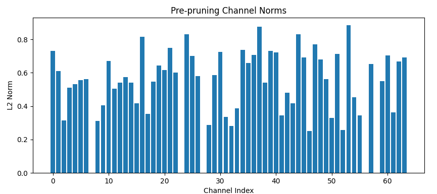

四、知识蒸馏实战
import torch
import torch.nn as nn
import torch.nn.functional as F
from torchvision import models
from torch.utils.data import DataLoader
from torchvision import datasets, transforms
from tqdm import tqdm
# 设备配置
device = torch.device("cuda" if torch.cuda.is_available() else "cpu")
# 1. 数据准备
transform = transforms.Compose([
transforms.Resize(256),
transforms.CenterCrop(224),
transforms.ToTensor(),
transforms.Normalize(mean=[0.485, 0.456, 0.406], std=[0.229, 0.224, 0.225]),
])
train_dataset = datasets.CIFAR100(
root='./data',
train=True,
download=True,
transform=transform
)
test_dataset = datasets.CIFAR100(
root='./data',
train=False,
download=True,
transform=transform
)
train_loader = DataLoader(train_dataset, batch_size=64, shuffle=True)
test_loader = DataLoader(test_dataset, batch_size=64, shuffle=False)
# 2. 模型初始化
def create_model(model_name, pretrained=False, num_classes=100):
"""创建并修改模型最后一层"""
model = models.__dict__[model_name](weights="DEFAULT" if pretrained else None)
if 'resnet' in model_name:
model.fc = nn.Linear(model.fc.in_features, num_classes)
elif 'convnext' in model_name:
model.classifier[-1] = nn.Linear(model.classifier[-1].in_features, num_classes)
return model.to(device)
# 教师模型 (ResNet152)
teacher = create_model('resnet152', pretrained=True, num_classes=100)
teacher.eval() # 教师模型固定参数
# 学生模型 (ResNet18)
student = create_model('resnet18', pretrained=False, num_classes=100)
# 3. 知识蒸馏损失
class DistillationLoss(nn.Module):
def __init__(self, T=2.0, alpha=0.7):
super().__init__()
self.T = T
self.alpha = alpha
self.ce_loss = nn.CrossEntropyLoss()
def forward(self, student_logits, teacher_logits, targets):
# 教师软标签
soft_teacher = F.softmax(teacher_logits/self.T, dim=1)
# 学生软预测
soft_student = F.log_softmax(student_logits/self.T, dim=1)
# 组合损失
kld_loss = F.kl_div(soft_student, soft_teacher, reduction='batchmean') * (self.T**2)
ce_loss = self.ce_loss(student_logits, targets)
return self.alpha * kld_loss + (1 - self.alpha) * ce_loss
# 4. 训练配置
criterion = DistillationLoss(T=3.0, alpha=0.7)
optimizer = torch.optim.AdamW(student.parameters(), lr=1e-4, weight_decay=0.01)
scheduler = torch.optim.lr_scheduler.CosineAnnealingLR(optimizer, T_max=20)
# 5. 训练循环
def train_one_epoch(model, teacher, loader, optimizer, criterion):
model.train()
total_loss = 0.0
for inputs, targets in tqdm(loader, desc="Training"):
inputs, targets = inputs.to(device), targets.to(device)
with torch.no_grad():
teacher_logits = teacher(inputs)
# 学生模型前向
student_logits = model(inputs)
# 计算损失
loss = criterion(student_logits, teacher_logits, targets)
# 反向传播
optimizer.zero_grad()
loss.backward()
optimizer.step()
total_loss += loss.item()
return total_loss / len(loader)
# 6. 评估函数
def evaluate(model, loader):
model.eval()
correct = 0
total = 0
with torch.no_grad():
for inputs, targets in tqdm(loader, desc="Evaluating"):
inputs, targets = inputs.to(device), targets.to(device)
outputs = model(inputs)
_, predicted = outputs.max(1)
total += targets.size(0)
correct += predicted.eq(targets).sum().item()
return 100 * correct / total
# 7. 完整训练流程
best_acc = 0.0
for epoch in range(20):
print(f"\nEpoch {epoch+1}/20")
# 训练
train_loss = train_one_epoch(student, teacher, train_loader, optimizer, criterion)
scheduler.step()
# 评估
val_acc = evaluate(student, test_loader)
# 保存最佳模型
if val_acc > best_acc:
best_acc = val_acc
torch.save(student.state_dict(), "best_student.pth")
print(f"New best model saved with accuracy: {best_acc:.2f}%")
print(f"Train Loss: {train_loss:.4f} | Val Acc: {val_acc:.2f}%")
# 8. 最终测试
student.load_state_dict(torch.load("best_student.pth", weights_only=True))
final_acc = evaluate(student, test_loader)
print(f"\nFinal Test Accuracy: {final_acc:.2f}%")输出为:
Epoch 1/20
Training: 100%|██████████████████████████████████████████████████| 782/782 [08:46<00:00, 1.49it/s]
Evaluating: 100%|████████████████████████████████████████████████| 157/157 [00:25<00:00, 6.14it/s]
New best model saved with accuracy: 22.92%
Train Loss: 1.2542 | Val Acc: 22.92%
Epoch 2/20
Training: 100%|██████████████████████████████████████████████████| 782/782 [08:49<00:00, 1.48it/s]
Evaluating: 100%|████████████████████████████████████████████████| 157/157 [00:25<00:00, 6.14it/s]
New best model saved with accuracy: 33.67%
Train Loss: 1.1239 | Val Acc: 33.67%
Epoch 3/20
Training: 100%|██████████████████████████████████████████████████| 782/782 [08:49<00:00, 1.48it/s]
Evaluating: 100%|████████████████████████████████████████████████| 157/157 [00:25<00:00, 6.14it/s]
New best model saved with accuracy: 39.92%
Train Loss: 1.0307 | Val Acc: 39.92%
Epoch 4/20
Training: 100%|██████████████████████████████████████████████████| 782/782 [08:50<00:00, 1.48it/s]
Evaluating: 100%|████████████████████████████████████████████████| 157/157 [00:25<00:00, 6.10it/s]
New best model saved with accuracy: 45.60%
Train Loss: 0.9532 | Val Acc: 45.60%
Epoch 5/20
Training: 100%|██████████████████████████████████████████████████| 782/782 [08:49<00:00, 1.48it/s]
Evaluating: 100%|████████████████████████████████████████████████| 157/157 [00:26<00:00, 5.97it/s]
New best model saved with accuracy: 50.02%
Train Loss: 0.8839 | Val Acc: 50.02%
......
Epoch 16/20
Training: 100%|██████████████████████████████████████████████████| 782/782 [08:49<00:00, 1.48it/s]
Evaluating: 100%|████████████████████████████████████████████████| 157/157 [00:25<00:00, 6.11it/s]
New best model saved with accuracy: 56.49%
Train Loss: 0.3927 | Val Acc: 56.49%
Epoch 17/20
Training: 100%|██████████████████████████████████████████████████| 782/782 [08:50<00:00, 1.47it/s]
Evaluating: 100%|████████████████████████████████████████████████| 157/157 [00:25<00:00, 6.16it/s]
Train Loss: 0.3848 | Val Acc: 56.45%
Epoch 18/20
Training: 100%|██████████████████████████████████████████████████| 782/782 [08:49<00:00, 1.48it/s]
Evaluating: 100%|████████████████████████████████████████████████| 157/157 [00:25<00:00, 6.12it/s]
New best model saved with accuracy: 56.60%
Train Loss: 0.3795 | Val Acc: 56.60%
Epoch 19/20
Training: 100%|██████████████████████████████████████████████████| 782/782 [08:50<00:00, 1.47it/s]
Evaluating: 100%|████████████████████████████████████████████████| 157/157 [00:25<00:00, 6.15it/s]
Train Loss: 0.3766 | Val Acc: 56.47%
Epoch 20/20
Training: 100%|██████████████████████████████████████████████████| 782/782 [08:50<00:00, 1.47it/s]
Evaluating: 100%|████████████████████████████████████████████████| 157/157 [00:25<00:00, 6.18it/s]
New best model saved with accuracy: 56.64%
Train Loss: 0.3748 | Val Acc: 56.64%
Evaluating: 100%|████████████████████████████████████████████████| 157/157 [00:28<00:00, 5.50it/s]
Final Test Accuracy: 56.64%五、模型部署优化
1. ONNX 导出
import torch
from torchvision import models

model = models.resnet50(weights=models.ResNet50_Weights.IMAGENET1K_V1)

dummy_input = torch.randn(1, 3, 224, 224)
torch.onnx.export(
    model,
    dummy_input,
    'model.onnx',
    opset_version=13,
    input_names=['input'],
    output_names=['output'],
    dynamic_axes={
        'input': {0: 'batch_size'},
        'output': {0: 'batch_size'}
    }
)

# 注意需要执行 pip install onnx
2. TensorRT 加速
# 转换ONNX到TensorRT
trtexec --onnx=model.onnx --saveEngine=model.engine \
        --fp16 --workspace=4096 --explicitBatch
3. 移动端部署(LibTorch)
// C++ 加载量化模型
torch::jit::Module module;
module = torch::jit::load("quantized_model.pt");
module.eval();

// 创建输入张量
std::vector<torch::jit::IValue> inputs;
inputs.push_back(torch::ones({1, 3, 224, 224}));

// 运行推理
auto output = module.forward(inputs).toTensor();
六、总结
本文介绍了以下核心内容:
量化技术:动态/静态量化的实现方法
模型剪枝:结构化与非结构化剪枝策略
知识蒸馏:教师-学生模型训练框架
部署优化:ONNX/TensorRT/LibTorch 部署流程
在下一篇文章《可解释性AI与特征可视化》中,我们将探索如何理解和解释深度学习模型的决策过程。
实践建议:
优先尝试动态量化(实现简单,无需重新训练)
高精度场景使用静态量化+校准
移动端部署推荐结合剪枝和量化
使用 TensorRT 实现极致推理加速